2 The Supervised Recipe
2.1 Simple Linear Regression
The first chapter ended with a map and no methods on it. Every node of Figure 1.49 names a family of problems, and that chapter fitted models to data only as worked examples. This section takes the simplest node that is still a complete learner and builds a learner on it, in full, for the first time: two columns of numbers, no formula available, and a prediction required.
The problem chosen is the most familiar one in the field. A house has not sold, and somebody needs to know what it is worth. A buyer needs the number to decide what to offer, since an offer too high loses money and an offer too low loses the house. A lender needs it because a mortgage is secured against a valuation, and a valuation set too high leaves the loan uncovered if the borrower stops paying. A tax assessor needs it because property tax is charged on an assessed value. Errors in the number are not abstract. In November 2021 Zillow Group announced that it would wind down Zillow Offers, its house-buying business, after writing down $304 million on homes it had bought for more than its own estimates now said they would sell for (Zillow Group, Inc. 2021).
The problem is familiar for a reason, and it is worth seeing why it belongs to this book before anything is fitted. The question concerns a system that cannot be experimented on: nobody can sell the same house ten times to see what happens, so the answer has to come from a model in the sense of Definition 1.1. Three questions then place it on Figure 1.49. There is no law that gives a house’s price in the way Newton’s law of cooling gives the temperature of a cup, so the form of the model must come from data. The price was recorded for houses that have already sold, so the data carries an answer column and the task is supervised in the sense of Definition 1.19. The answer is a number, so the task is regression by Definition 1.21. Figure 2.1 draws the three answers and the address they build.
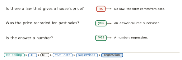
The examples in this section are real sales. De Cock assembled the Ames housing data from the records of the city assessor of Ames, Iowa, and published it in the Journal of Statistics Education in 2011 as an alternative to the older Boston housing data for teaching regression (De Cock 2011). It holds 2,930 residential sales from 2006 to 2010, each described by about eighty recorded columns. Its documentation flags five sales with more than 4,000 square feet of living space, three of them partial sales of unfinished houses and two of them very large houses, and recommends removing them. We follow that advice, and we hold one further sale back from every fit so that it can be predicted honestly later. It is a house of 134 square metres, built in 1968, that sold in 2010. That leaves 2,924 sales.
Living area is converted to square metres at 0.0929 square metres to the square foot, and prices are given in thousands of dollars. Throughout the section \(x_i\) is the living area of sale \(i\) in square metres, \(y_i\) is its price in thousands of dollars, and \(n = 2{,}924\). The averages are \(\bar{x} = 138.8\) m² and \(\bar{y} = 180.4\) thousand dollars.
The problem can now be stated precisely. Estimate a house’s price from what is recorded about it, using houses that have sold. This section makes one simplification and keeps it to the end.
Definition 2.1 (Simple regression) Simple regression is regression with one input column. The word simple refers to the number of inputs and to nothing else.
With one input fixed, the work divides into two tasks that are different in kind. The first is to decide how the world works: what form the relationship between price and area takes. Whatever is decided there is an assumption. The data can support it or contradict it, but the data does not hand it over. The second task is to find, inside that form, the member that fits the recorded sales best, and that answer is computed. The two tasks are the three choices of Definition 1.16 in a different grouping. The first task is the hypothesis space. The second is the loss and the optimiser together.
Task one: how the world works
The assessor recorded about eighty columns for every sale, and simple regression uses one of them. Figure 2.2 plots price against five candidates for the same random thousand sales. Living area shows a strong rise that looks roughly straight. The quality rating rises steeply too, but it is a judgement on a scale from one to ten rather than a measurement, and its points fall in stripes. Year built rises along a curve, flat for decades and then climbing. Lot area cannot be read at all, because a handful of enormous lots stretch the axis and crush every other point into one corner. The month of sale shows no relation to price.
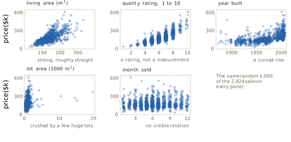
We choose living area, because its rise is strong and looks straight. The method of choosing matters as much as the choice. We looked at the data and decided by eye, which is exploratory data analysis in the sense that Tukey gave the phrase (Tukey 1977) and that Section 1.3 placed inside statistics and data science. Choosing among many inputs by a method rather than by eye is taken up in Sections 2.2 and 2.7, and the related question of which inputs a fitted model relies on in Section 5.7.
With the input chosen, the hypothesis space has to be chosen too. Four families are natural candidates, and each is a whole set of functions rather than one function:
\[ \begin{aligned} &\text{constant:} && y = b, \\ &\text{linear:} && y = b + w\,x, \\ &\text{quadratic:} && y = b + w_1 x + w_2 x^2, \\ &\text{higher order:} && y = b + w_1 x + w_2 x^2 + \cdots + w_k x^k . \end{aligned} \tag{2.1}\]
In the constant family the price does not depend on area at all. In the linear family every extra square metre adds the same amount \(w\), and changing \(b\) moves the line up or down while changing \(w\) tilts it. The quadratic family lets the rise itself grow or shrink with size, so its members can bend once. The higher-order family can bend as often as its order allows. The families are nested: every constant is a line with \(w = 0\), every line is a quadratic with \(w_2 = 0\), and so on upward.
The linear, quadratic and cubic families are fitted in Figure 2.3 to all 2,924 sales by least squares and overlaid. Inside the range of the data neither curved fit departs from the straight line by more than $13 thousand, and the two curves differ from each other by at most $16 thousand, at the largest house. Beyond the largest house sold they part company, and at 450 square metres the highest and the lowest of the three disagree by $69 thousand, in a region where no recorded sale can settle which is right.
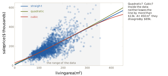
We therefore assume that the world is a straight line. The word assume is chosen with care. Nothing in Figure 2.3 proves the relationship linear, and a more flexible family always follows the recorded points at least as closely as the line does, because it contains the line. Following the points more closely is not a reason to choose a family. Why it is not is the subject of Sections 2.3 and 2.7.
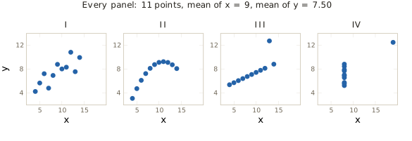
That the shape must be looked at, and cannot be computed from a summary, was put beyond argument by Anscombe in Graphs in Statistical Analysis, published in The American Statistician in 1973 (Anscombe 1973). He constructed four small datasets of eleven points each. All four have a mean of \(x\) equal to 9 and a mean of \(y\) equal to 7.50, and they share much more besides. The least-squares line through each is \(\hat{y} = 3.00 + 0.500\,x\), and the line explains the same fraction of the variation in each. Figure 2.4 plots them. The first is a fair scatter about a straight rise. The second is a smooth curve, for which a straight line is the wrong form. The third lies exactly on a line except for one record. In the fourth, ten points share one value of \(x\) and a single distant point creates the appearance of a trend. Four shapes that call for four different responses produce identical numbers.
The true model and its estimate
The assumption can now be written as an equation, and the way it is written separates what we claim about the world from what we compute.
Definition 2.2 (True model) The true model of simple linear regression asserts that \[ y_i \;=\; b + w\,x_i + \varepsilon_i , \qquad i = 1, \ldots, n , \tag{2.2}\] where \(b\) and \(w\) are fixed numbers, the same for every house, and the error term \(\varepsilon_i\) is everything about sale \(i\) that the line leaves out.
The quantities in Equation 2.2 are the world’s. The intercept \(b\) and the slope \(w\) are not known and never will be. The model supplies a structure with two slots and asserts that true values fill them. The error term holds the build quality, the neighbourhood, the condition of the roof, the day of the sale and how hard the buyer bargained, and it is unknown for every sale. Adding columns can shrink it but cannot empty it, since there is always something about a sale that the equation does not capture. That is the content of Box’s remark, discussed in Section 1.1, that all models are wrong (Box 1976).
What we compute from the sales are estimates, and they are marked with a hat. The estimates \(\hat{b}\) and \(\hat{w}\) approximate \(b\) and \(w\), and the price the fitted line predicts for a house of area \(x\) is
\[ \hat{y} \;=\; \hat{b} + \hat{w}\,x . \tag{2.3}\]
The estimate in Equation 2.3 carries no error term. A fitted line predicts a price, and it makes no claim to account for everything. The convention holds for the rest of this book: no hat on what the world is, and a hat on what we compute to approximate it.
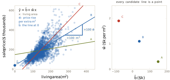
Every choice of the pair \((\hat{b}, \hat{w})\) is one candidate line. The slope \(\hat{w}\) is the rise in predicted price per extra square metre, so that moving 100 square metres to the right raises the line by \(100\,\hat{w}\). The intercept \(\hat{b}\) is where the line meets zero area. No house has zero area, so \(\hat{b}\) is where the line lands rather than a price anybody paid. Plotting each candidate’s two numbers as a point turns the hypothesis space into a plane, which Figure 2.5 draws for three candidates. Somewhere on that plane is the point \((b, w)\), and we will never see exactly where.
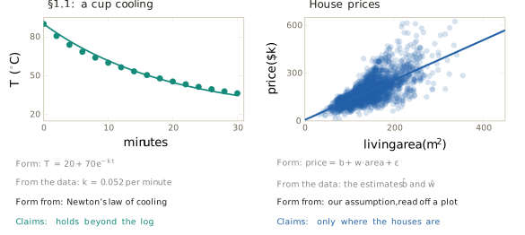
An objection has to be answered before the search begins. Fitting \(b\) and \(w\) by least squares is the same arithmetic that Section 1.1 used to fit the cooling constant \(k\), and Section 1.1 said that fitting \(k\) was numerical computation rather than machine learning. What makes the same arithmetic learning here is the origin of the form and the reach of the claim. The form of the cooling curve came from Newton’s law, and only one constant was left to fill. The straight line came from an assumption read off a plot, chosen from a space of candidates. The cooling law claims to hold beyond the log, because it is a law. The fitted line claims only to be a fair guide to houses like these, inside the range already seen, and that is still a claim about houses not yet sold. Figure 2.6 sets the two fits side by side.
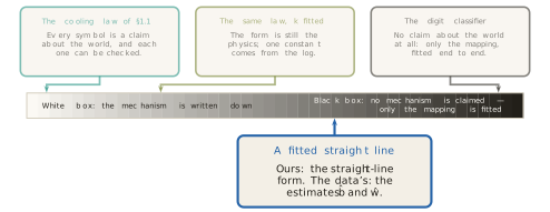
The modelling axis of Figure 1.36 runs from a white box, where the mechanism is written down and every symbol is a claim about the world, to a black box, where no mechanism is claimed and only the mapping from input to output is fitted. The cooling law sits at the white end. The same law with \(k\) fitted to the log sits just inside it, because the form is still the physics. A classifier of handwritten digits, fitted end to end, sits near the black end, and not on it. The fitted line sits well into the interior. The straight-line form is ours, and the two numbers are the data’s. Figure 2.7 places it, the first method to receive a position on that axis.
Task two: a score, then a search
The form is now fixed, and task two asks which of its members fits best. That question has two parts: what best means, which is the loss, and how the best member is found, which is the optimiser. The loss comes first, since nothing can be searched for until candidates can be compared.
A line misses each recorded sale by some amount. The miss is measured vertically, as the recorded price minus the predicted price, because price is the quantity predicted and an error in area is of no interest. Squaring each miss and adding the squares gives one number for each candidate line.
Definition 2.3 (Residual sum of squares) The residual sum of squares (RSS) of a candidate line is \[ \mathrm{RSS}(\hat{b}, \hat{w}) \;=\; \sum_{i=1}^{n} \bigl( y_i - (\hat{b} + \hat{w}\,x_i) \bigr)^2 . \tag{2.4}\]
The score in Equation 2.4 is the empirical risk of Equation 1.19 with the squared loss of Equation 1.26, written for candidate lines and multiplied by \(n\). The factor changes the size of the score and leaves the order of the candidates unchanged, so the line that minimises one minimises the other. It is also Equation 1.7 with two constants in place of one. The idea is least squares in the sense of Definition 1.4, published by Legendre in 1805 (Legendre 1805) and by Gauss in 1809 (Gauss 1809), as Section 1.1 told.
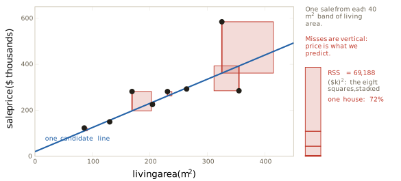
A small worked case shows what the score is made of. Take eight sales, one from each band of forty square metres between 60 and 380 square metres, and the candidate line \(\hat{y} = 20 + 1.05\,x\), which is not the best line and was not chosen to be. Each miss is squared and drawn as a square at true scale in Figure 2.8, and the eight squares are stacked into one bar. The total is 69,188 in units of thousands of dollars squared. Nobody can picture that unit, and nothing requires it, because RSS totals are only ever compared with each other. What the bar shows clearly is the split. The sale at 325 square metres sold for $584.5 thousand, the line predicts $361.4 thousand there, and that one miss of $223 thousand is 72% of the whole score.
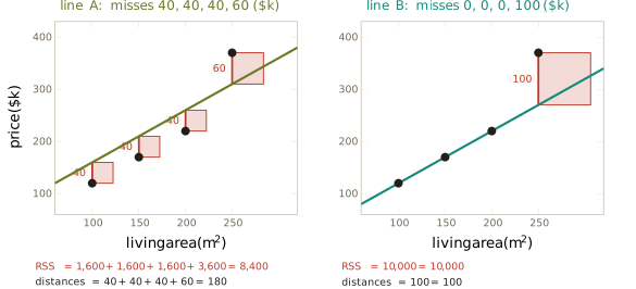
The 72% is not an accident of the example. Squaring makes the cost of a miss grow with the square of its size, so a miss ten times larger costs a hundred times more, and one large miss can outweigh many small ones. Two lines through the same four houses make the consequence concrete. Line A misses them by 40, 40, 40 and 60 thousand dollars. Line B passes exactly through three of them and misses the fourth by 100 thousand. Under squares, line A scores \(1{,}600 + 1{,}600 + 1{,}600 + 3{,}600 = 8{,}400\) and line B scores \(10{,}000\), so squares prefer A. Under the sum of distances, A scores 180 and B scores 100, so distances prefer B. Figure 2.9 draws both. The same houses under two losses produce two different winners, and the squared loss prefers many small misses to one large one.
On the Ames data the cost of this preference is visible in the five sales the documentation flags. With them restored there are 2,929 sales, and the five carry 6.8% of the whole RSS between them. They pull the fitted slope from $1,251 per square metre down to $1,202, as Figure 2.10 shows.
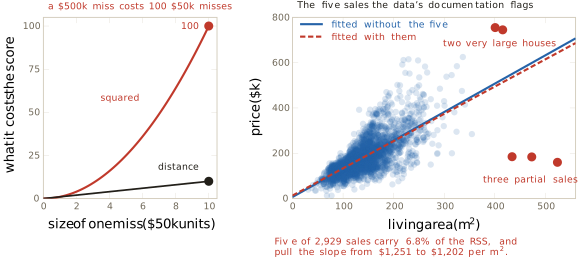
Squares are chosen nonetheless, for what they buy. The score they produce is a smooth surface over the plane of candidates with a single lowest point, which the next part of this section draws, and that makes the search tractable. What they cost returns when outliers are examined at the end of the section, and Section 2.5 gives the squared loss a justification from probability that this section does not need.
With a score in hand, the search can begin. The plainest search tries a grid of candidates and keeps the best. Before running it we change the units in which area is measured, which changes how the two numbers read and changes nothing about the lines. Let
\[ u_i \;=\; \frac{x_i - \bar{x}}{100} , \tag{2.5}\]
the area of sale \(i\) measured from the average house in hundreds of square metres, and write the candidate line as \(\hat{y} = \hat{b} + \hat{w}\,u\). In these units \(\hat{b}\) is the predicted price of a house of average size, around $180 thousand, and \(\hat{w}\) is the rise in thousands of dollars per extra hundred square metres, so a slope of $1.25 thousand per square metre reads as 125. We keep the names \(\hat{b}\) and \(\hat{w}\) for the pair in these units, and every figure from here to the closed form uses them; where the everyday pair is needed it carries a subscript 0. A line written in everyday units as \(\hat{b}_0 + \hat{w}_0 x\) is the same line as \(\hat{b} + \hat{w}\,u\) exactly when \(\hat{w} = 100\,\hat{w}_0\) and \(\hat{b} = \hat{b}_0 + \hat{w}_0\,\bar{x}\). The reason for the change is practical. In raw units the two parameters live on scales so different that the score’s curvature, the rate at which its slope changes, is about 222,000 times greater along the steepest direction of the plane than along the direction at right angles to it. The bowl is a long thin trough, and that is a difficulty for Section 2.4 rather than for this one. One property of the new units is used repeatedly below: because each \(u_i\) is a distance from the average,
\[ \sum_{i=1}^{n} u_i \;=\; 0 . \tag{2.6}\]
Two loops then perform the search. The intercept runs from 100 to 260 in steps of 10, giving 17 values, and the slope from 0 to 250 in steps of 10, giving 26 values. Every one of the \(17 \times 26 = 442\) pairs is scored by Equation 2.4 and the best is kept. It is \((\hat{b}, \hat{w}) = (180, 130)\), a line that runs through the middle of the cloud of sales, and its RSS is 0.17% above the lowest possible. Two loops work.
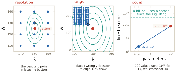
Their costs are three, and Figure 2.11 draws them side by side. The first is resolution. The true bottom lies between grid points, so the best grid point misses it, and moving closer requires a finer grid and more lines to score. The second is range. The loops search only where they are told to, and a grid placed wrongly returns a best point on its own edge, here 18% above the bottom, with no sign that anything is amiss. The third is the count. With 100 values for each of \(p\) parameters the grid holds
\[ N(p) \;=\; 100^{\,p} \tag{2.7}\]
lines. Two parameters give \(10^4\) lines and ten give \(10^{20}\), which at a billion lines a second takes about 3,200 years. Every line a billion-a-second machine could have scored since the Big Bang, roughly \(4 \times 10^{26}\) of them, is exceeded at fourteen parameters. This is the candidate count of Section 1.3 met again, now in a problem with only two parameters where it can still be paid.
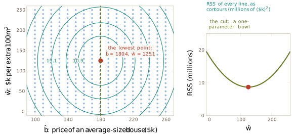
Every point of the plane is a line and every line has a score, so the score is a surface over the plane. Figure 2.12 draws it from above as contours, like a map of a valley. The contours are closed rings around one lowest point, at \(\hat{b} = 180.4\) and \(\hat{w} = 125.1\). A straight cut through that point with \(\hat{b}\) held fixed gives a curve with one bottom, which is the one-parameter bowl of Figure 1.33. The two-parameter score is the same object in two directions. Seen in three dimensions it is a bowl, and the contour map is that bowl seen from directly above.
That the surface is a bowl with exactly one bottom is not a feature of these data, and a few lines of algebra show why. Write \(S_{uu} = \sum u_i^2\), \(S_{uy} = \sum u_i y_i\) and \(S_{yy} = \sum (y_i - \bar{y})^2\). In Equation 2.4 with centred area, split each \(y_i - \hat{b}\) as \((y_i - \bar{y}) + (\bar{y} - \hat{b})\) and expand the square. Three cross terms appear. One carries \(\sum (y_i - \bar{y})\), which is zero because deviations from a mean add to zero. One carries \(\sum u_i\), which is zero by Equation 2.6. The third carries \(\sum u_i (y_i - \bar{y})\), which by Equation 2.6 is \(S_{uy}\). Completing the square in \(\hat{w}\) then gives
\[ \mathrm{RSS}(\hat{b}, \hat{w}) \;=\; n\,(\hat{b} - \bar{y})^2 \;+\; S_{uu}\Bigl(\hat{w} - \frac{S_{uy}}{S_{uu}}\Bigr)^2 \;+\; \Bigl(S_{yy} - \frac{S_{uy}^2}{S_{uu}}\Bigr) . \tag{2.8}\]
The last bracket does not depend on the candidate. The first two terms are squares with positive coefficients (\(S_{uu}\) is positive unless every house has the same area), so they are never negative and are both zero at exactly one point. The score is therefore a sum of two upward parabolas, one in each direction, and it has one bottom and nowhere else flat. On the Ames data \(n = 2{,}924\) and \(S_{uu} = 596.76\), so the bowl curves about five times more steeply along \(\hat{b}\) than along \(\hat{w}\), which is why the contours of Figure 2.12 are ellipses stretched along the \(\hat{w}\) axis. The same algebra applies to any subset of the sales, with area measured from that subset’s own average, and that settles a question about the amount of data.
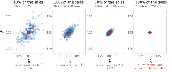
The bowl was built from all 2,924 sales. Built from a random 10% of them, 292 houses, it is still a smooth bowl with one bottom, and Equation 2.8 applied to those 292 houses says it must be. Drawn in the coordinates of the full data the bowl is tilted, since the subset’s average area is not exactly 138.8, but tilting does not add a second bottom. What changes is where the bottom lies. On one nested sequence of samples, 10%, 30%, 70% and all of the sales put the bottom’s \(\hat{w}\) at 114.0, 122.5, 124.7 and 125.1. Repeating the 10% draw two hundred times scatters the bottoms widely. Measured by the standard deviation across the two hundred draws, \(\hat{w}\) varies by about 9.6 and \(\hat{b}\) by about 3.0. At 30% the standard deviation of \(\hat{w}\) is about 4.6, and at 70% about 2.2. With every sale, every draw is the same set of houses, so there is one answer. Figure 2.13 shows the four clouds. More data does not smooth this bowl, since the bowl is smooth at any size. It fixes where the bottom is. Even with all 2,924 sales the bottom gives estimates of \(b\) and \(w\) and not the values themselves, and Section 2.6 gives the spread across samples its name and its law.
Finding the bottom
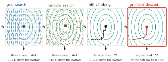
There is more than one way down a bowl, and racing four of them on this one shows what each costs. Figure 2.14 reports for each search how much work it did and how close it ended. Grid search scores 442 lines and ends 0.17% above the bottom. Random search, with the same budget of 442 lines placed at random, ends 0.69% above, which is worse for the same work. Hill climbing, met in Section 1.2, stands at a point, scores its four neighbours one grid step away, moves to the best and repeats. It scores 73 lines and stops on the same grid point as the grid, because its steps are the grid’s size. Gradient descent scores no neighbours at all. It reads the slope where it stands and steps downhill, and after reading the slope 60 times it ends at the bottom to within 0.01%. Evolutionary search, also met in Section 1.2, is left out of the race. So is the exact answer, which this section reaches after gradient descent.
Gradient descent was introduced in Section 1.3 on a bowl of one parameter, with the slope taken as given. Taking it apart in two parameters needs the slope itself made precise, and the clearest place to do that is a curve of one parameter that has both a top and a bottom.
Standing at one point of a curve \(f(\theta)\), there are only two moves: make \(\theta\) larger, or make it smaller. The slope decides which of the two goes down. It is a signed number. Its sign is a direction and its size is a steepness. A positive slope means that \(f\) increases as \(\theta\) increases, so uphill is to the right and downhill to the left. A negative slope means the reverse. At a top or a bottom the slope is zero and points nowhere, which is how a top or a bottom is recognised. Following the slope climbs, and going against it descends, so the two rules differ only in a sign:
\[ \text{climb: } \theta \leftarrow \theta + \eta \cdot \text{slope}, \qquad \text{descend: } \theta \leftarrow \theta - \eta \cdot \text{slope} , \tag{2.9}\]
where the step size \(\eta\) is chosen in advance. Because a step proportional to the slope is long where the ground falls fast and short where it flattens, the descent slows as it approaches a bottom of its own accord.
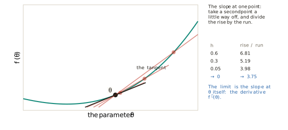
What remains is how the slope at a point is computed. One point has neither a rise nor a run, so a second point is taken a distance \(h\) away and the rise is divided by the run. That ratio is the slope of the secant, the straight line through both points, and it is the average slope between them. Shrinking \(h\) moves the second point towards the first, and the ratio settles on a single value.
Definition 2.4 (Derivative) The derivative of \(f\) at \(\theta\) is \[ f'(\theta) \;=\; \lim_{h \to 0} \frac{f(\theta + h) - f(\theta)}{h} , \tag{2.10}\] the slope of the curve at the point \(\theta\) itself. The secant through \(\theta\) and \(\theta + h\) becomes, in the limit, the tangent at \(\theta\).
The curve of Figure 2.15 is \(f(\theta) = \theta^3 - 3\theta\), and the point is \(\theta = 1.5\). The rise over a run of \(h\) is
\[ \frac{f(1.5 + h) - f(1.5)}{h} \;=\; \frac{(1.5 + h)^3 - 3(1.5 + h) - (1.5^3 - 4.5)}{h} \;=\; 3.75 + 4.5\,h + h^2 , \tag{2.11}\]
after expanding the cube and dividing by \(h\). At \(h = 0.6\) the ratio is 6.81, at \(h = 0.3\) it is 5.19, and at \(h = 0.05\) it is 3.98. As \(h\) goes to zero the two terms that carry \(h\) vanish, and the derivative is \(f'(1.5) = 3.75\). The same expansion at a general \(\theta\) gives \(f'(\theta) = 3\theta^2 - 3\), which is zero at \(\theta = -1\) and \(\theta = 1\), the top and the bottom of the curve. The idea goes back to Newton and Leibniz in the late seventeenth century, and the limit in Equation 2.10 was made precise in the nineteenth. From here on, the slope at a point means the derivative there.
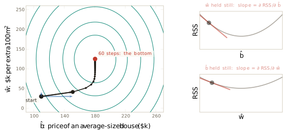
The RSS has two parameters, so a single slope does not describe it. Holding one parameter still and letting the other move cuts the bowl along one direction and returns the problem to one dimension.
Definition 2.5 (Partial derivative and gradient) A partial derivative is the derivative along one parameter while every other parameter is held still. For the score of Equation 2.4 they are written \(\partial\,\mathrm{RSS}/\partial \hat{b}\) and \(\partial\,\mathrm{RSS}/\partial \hat{w}\). The gradient is the vector of all the partial derivatives, \[ \nabla \mathrm{RSS} \;=\; \Bigl( \frac{\partial\,\mathrm{RSS}}{\partial \hat{b}},\; \frac{\partial\,\mathrm{RSS}}{\partial \hat{w}} \Bigr) . \tag{2.12}\]
Each entry of Equation 2.12 is the slope in its own direction, and together they point uphill. The symbol \(\nabla\) was used in Equation 1.21 as a name for the slope, and Definition 2.5 is what the name means.
Both partial derivatives of the RSS follow from Equation 2.10 alone. Write the miss of sale \(i\) as \(r_i = y_i - \hat{b} - \hat{w}\,u_i\). Moving \(\hat{b}\) by \(h\) changes the miss to \(r_i - h\), and its square changes by \((r_i - h)^2 - r_i^2 = -2h\,r_i + h^2\). Dividing by \(h\) and letting \(h\) go to zero leaves \(-2r_i\). Moving \(\hat{w}\) by \(h\) changes the miss to \(r_i - h\,u_i\), and the same steps leave \(-2u_i r_i\). Adding over the sales gives
\[ \frac{\partial\,\mathrm{RSS}}{\partial \hat{b}} \;=\; -2 \sum_{i=1}^{n} \bigl( y_i - \hat{b} - \hat{w}\,u_i \bigr), \qquad \frac{\partial\,\mathrm{RSS}}{\partial \hat{w}} \;=\; -2 \sum_{i=1}^{n} u_i \bigl( y_i - \hat{b} - \hat{w}\,u_i \bigr) . \tag{2.13}\]
Section 2.2 derives the same result for any number of inputs. Descent goes against the gradient, and the whole method fits on one line.
Definition 2.6 (Gradient descent on the RSS) Start at any candidate \((\hat{b}, \hat{w})\). Compute the gradient there by Equation 2.13, and step against it: \[ (\hat{b}, \hat{w}) \;\leftarrow\; (\hat{b}, \hat{w}) \;-\; \eta\, \nabla \mathrm{RSS}(\hat{b}, \hat{w}) . \tag{2.14}\] Stop when both partial derivatives are near zero; otherwise compute the gradient again.
The update in Equation 2.14 is Equation 1.21 with \(\theta\) standing for two numbers at once. Cauchy published the method in the Comptes Rendus in 1847 (Cauchy 1847), as Section 1.3 recorded. On the Ames bowl, with \(\eta = 0.0001\) and a start at \((110, 30)\), sixty passes of the loop reach \((180.4, 125.1)\). Figure 2.16 draws the path together with the two cuts whose slopes give the first step.
One step can be worked by hand, from a candidate at the upper right of the plane, \(\hat{b} = 240\) and \(\hat{w} = 200\). By Equation 2.13 and Equation 2.6 the first partial derivative is \(-2(n\bar{y} - n\hat{b})\), which is \(-2 \times 2{,}924 \times (180.4175 - 240) = +348{,}438\). The second is \(-2(S_{uy} - \hat{w}\,S_{uu})\), with \(S_{uy} = 74{,}655.9\) and \(S_{uu} = 596.756\), which is \(+89{,}391\). Multiplying each by \(\eta = 0.0001\) gives steps of 34.84 and 8.94, and subtracting them gives
\[ \hat{b} \;=\; 240 - 34.84 \;=\; 205.2, \qquad \hat{w} \;=\; 200 - 8.94 \;=\; 191.1 . \tag{2.15}\]
Both partial derivatives were positive, so both numbers fell, and the RSS dropped from 22.4 million to 13.1 million. Moving against the gradient is all that gradient descent ever does.
The path in Figure 2.16 bends rather than heading straight for the bottom, and Equation 2.8 explains why. Because \(\sum u_i = 0\), the update of \(\hat{b}\) involves only \(\hat{b}\) and the update of \(\hat{w}\) involves only \(\hat{w}\). Each step multiplies the distance of \(\hat{b}\) from its best value by \(1 - 2n\eta = 0.42\), and the distance of \(\hat{w}\) from its best value by \(1 - 2S_{uu}\eta = 0.88\). The intercept settles within a few steps, and the slope takes the rest of the sixty. The same factors show that the step size cannot be chosen freely: a factor larger than one in size makes each step overshoot further than the last. How to choose \(\eta\) well is the subject of Section 2.4.
Gradient descent earns its place by four properties, and the comparison with the grid makes them plain. It scores nothing but the point where it stands: the grid scored 442 lines, and descent reads two slopes and moves. Its cost does not grow with a grid, since there is no resolution to pick and no range to guess, although a step size and a starting point remain to be chosen. It scales: one slope per parameter means two here and millions in a neural network, against the \(10^{20}\) lines a grid would need for ten parameters. On this bowl it cannot be misled, because Equation 2.8 has one bottom and nowhere else is flat, so downhill leads to the same place from any start. Surfaces with more than one valley exist, and they are taken up in Section 2.4.
Solving instead of walking
The bottom of the bowl is the one point where both partial derivatives are zero, and for this model the partial derivatives are formulas. Rather than walking to the place where the slopes vanish, we can ask directly where that is. Setting both expressions of Equation 2.13 to zero gives two equations in two unknowns:
\[ \sum_{i=1}^{n} \bigl( y_i - \hat{b} - \hat{w}\,u_i \bigr) \;=\; 0, \qquad \sum_{i=1}^{n} u_i \bigl( y_i - \hat{b} - \hat{w}\,u_i \bigr) \;=\; 0 . \tag{2.16}\]
Measuring area from the average house makes the equations come apart. By Equation 2.6 the first reduces to \(n\bar{y} - n\hat{b} = 0\), and the second to \(S_{uy} - \hat{w}\,S_{uu} = 0\). So
\[ \hat{b} \;=\; \bar{y} \;=\; 180.4, \qquad \hat{w} \;=\; \frac{\sum_i u_i\, y_i}{\sum_i u_i^2} \;=\; 125.1 , \tag{2.17}\]
the same point that sixty steps of descent approached, reached with no steps at all. Equation 2.8 confirms from the other side that this point is the minimum and not merely a flat place, since both squared terms vanish there and nowhere else.
Converting back to everyday units with \(\hat{w}_0 = \hat{w}/100\) and \(\hat{b}_0 = \hat{b} - \hat{w}_0\,\bar{x}\), and dropping the subscripts, gives the formulas in the form they are usually printed.
Definition 2.7 (Least-squares line) The least-squares line through the points \((x_i, y_i)\) has slope and intercept \[ \hat{w} \;=\; \frac{\sum_i (x_i - \bar{x})(y_i - \bar{y})}{\sum_i (x_i - \bar{x})^2}, \qquad \hat{b} \;=\; \bar{y} - \hat{w}\,\bar{x} . \tag{2.18}\]
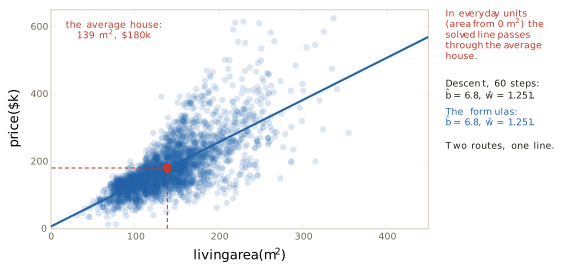
The second formula says that the least-squares line passes through the point of averages \((\bar{x}, \bar{y})\), the average house. On the Ames data that point is 138.8 square metres at $180.4 thousand, the slope is \(\hat{w} = 1.251\) thousand dollars per square metre, and the intercept is \(\hat{b} = 6.78\). Descent after sixty steps and the formulas give the same line, as Figure 2.17 shows. The formulas follow from the normal equations of Legendre and Gauss. Pearson, in the third of his Mathematical Contributions to the Theory of Evolution, published in the Philosophical Transactions of the Royal Society in 1896 (Pearson 1896), gave the product-moment correlation coefficient. He wrote the regression slope as that coefficient times the ratio of the two standard deviations, which is the same ratio of sums. The word regression is older. Galton used it in 1886 for the tendency of children’s heights to fall back towards the average (Galton 1886), as Section 1.4 described.
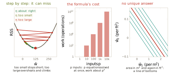
An answer that can be written down and computed in one pass is called a closed form. It exists for this model and for very few others in this book, and the comparison with stepping explains why the book mostly steps. Figure 2.18 sets out the trade. Stepping only approaches the answer, and how well depends on the step size. On the cut along \(\hat{w}\), a step size about right reaches the bottom in a few steps. One too small has barely moved after ten, and one too large overshoots further at every step and climbs out of the bowl. The formula is exact, but with \(p\) inputs it means solving \(p\) equations at once. The standard route goes through a table of \(p \times p\) numbers, a matrix, that must be inverted, and the work grows like \(p^3\), so ten times the inputs costs a thousand times the work and ten thousand inputs cost about \(10^{12}\) operations for one fit. And sometimes there is no single answer to compute. Suppose living area is entered twice, once in square metres and once in square feet. The two inputs carry the same information, so the score depends only on a combination of their two weights, and every point along a line of candidates is a bottom. The generalised inverse that Penrose defined in 1955 (Penrose 1955) picks one of those answers, but when two inputs are nearly rather than exactly equal it magnifies rounding error and the weights it returns can be badly wrong. Section 2.2 makes the matrix, the inverse and the failure precise. Stepping is cheap per step, works for any loss that has a slope, and scales to millions of parameters, and its price is that it only approaches the bottom.
Reading the fitted line
The fitted line is
\[ \hat{y} \;=\; 6.78 + 1.251\,x , \tag{2.19}\]
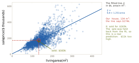
with \(\hat{y}\) in thousands of dollars and \(x\) in square metres. The house held back at the start has 134 square metres of living space, and Equation 2.19 predicts $174 thousand for it. It sold for $163 thousand. Because the sale was excluded from the fit, that is a genuine prediction, and it is $11 thousand too high.
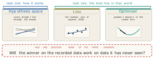
All three choices of Definition 1.16 have now been made on a real problem. The hypothesis space is every straight line in area. The loss is the residual sum of squares. The optimiser is gradient descent or the closed form. Figure 2.20 shows the filled card. This is the smallest complete learner, and every later method in this book can be read as a substitution into one or more of its slots. The question printed beneath the card is still open: whether the line that wins on the recorded sales will do well on sales it has never seen. Section 2.8 answers it.
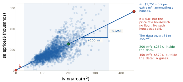
Each of the two numbers has a reading, and each reading has a limit. The slope says that, among these houses, each extra square metre goes with $1,251 more in price. The phrase among these houses matters, because the slope describes how price and area vary together in Ames between 2006 and 2010, and it says nothing about what adding a room to a particular house would do. The intercept, $6.78 thousand, is not the price of a house with no floor, and no such house was ever sold. It is where the line meets zero area. The recorded areas run from 31 to 355 square metres. A prediction at 200 square metres, $257 thousand, lies inside that range. A prediction at 450 square metres, $570 thousand, lies outside it and is a guess, which is the point Section 1.1 made about a fitted model that interpolates. Figure 2.21 marks both.
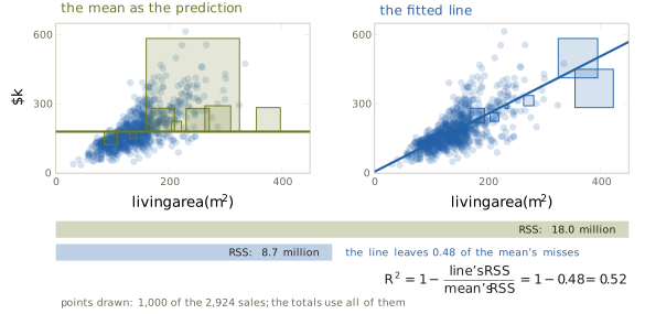
How good the line is depends on what it is compared with, and the natural baseline is the simplest predictor available: the average price for every house, whatever its area. That predictor is the constant family of Equation 2.1 at its best, and its score is \(S_{yy} = \sum (y_i - \bar{y})^2 = 18.0\) million. The fitted line scores 8.7 million, so it leaves 0.48 of the baseline’s squared misses.
Definition 2.8 (Coefficient of determination) The coefficient of determination of a fitted line is \[ R^2 \;=\; 1 - \frac{\mathrm{RSS}(\hat{b}, \hat{w})}{\sum_i (y_i - \bar{y})^2} , \tag{2.20}\] the fraction of the squared variation about the mean that the line accounts for.
For the Ames line \(R^2 = 1 - 0.48 = 0.52\). Living area explains about half the variation in price, and half is left. Wright introduced the name in Correlation and Causation, published in the Journal of Agricultural Research in 1921 (Wright 1921). The number is printed by every regression report, and it is often read as more than it is. Each of Anscombe’s four datasets has \(R^2 = 0.67\) under its fitted line, including the curve and the dataset whose trend is made by a single point. The number cannot tell them apart, and the plots of Figure 2.4 can.
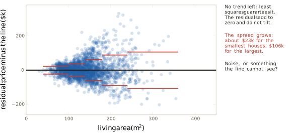
What the line leaves behind is its residuals, \(r_i = y_i - \hat{y}_i\) in the sense of Definition 1.3. A residual is not the error term \(\varepsilon_i\) of Equation 2.2. The error term is the miss of the true line, which is never seen, and the residual is the miss of the fitted line, which is computed. Figure 2.23 plots the residuals against living area. No straight-line trend remains, and least squares guarantees that much and no more: the two equations of Equation 2.16 say precisely that the residuals add to zero and that they do not tilt against area. A curved trend could survive them, as Anscombe’s second dataset would show, and none is visible here. What does remain is a change of spread. Measured by the standard deviation of the residuals within a band of sizes, the typical residual is about $23 thousand for houses between 40 and 100 square metres and about $106 thousand for those between 240 and 360. A single figure for the typical miss of the line would flatter it for small houses and mislead for large ones.
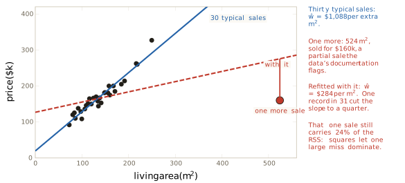
The cost of squaring, set aside earlier, can now be measured on a single record. Take thirty typical sales, one from the middle of each size band, and fit a line to them. Its slope is $1,088 per square metre. Add one more sale: 524 square metres, sold for $160 thousand, one of the five sales the documentation flags, a partial sale of a very large unfinished house. Refitted with it, the slope falls to $284 per square metre. One record in thirty-one has cut the slope to about a quarter, and after pulling the line towards itself that record still carries 24% of the RSS. One large miss counts for more than many small ones, so the line bends to shrink it. Figure 2.24 draws the two lines.
Definition 2.9 (Outlier) An outlier is a record that lies far from the pattern of the rest of the data. Under the squared loss it can have a large influence on the fit, the more so the further its input lies from the average.
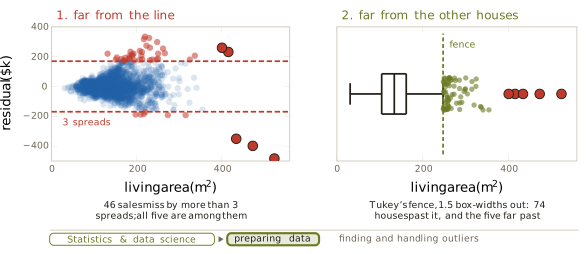
Two common rules find candidates, and Figure 2.25 applies both to all the sales with the five flagged ones restored. The first is distance from the line. Fit the line, take each residual, and flag any that exceeds three times the standard deviation of the residuals, here 3 × $56.5 thousand. Forty-six sales are flagged, and all five documented sales are among them. The second needs no line at all and asks how far a house is from the other houses. Tukey’s box plot, from Exploratory Data Analysis of 1977 (Tukey 1977), draws a box from the lower quartile \(Q_1\) to the upper quartile \(Q_3\) of living area, so that the box holds the middle half of the houses, and sets fences at
\[ Q_1 - 1.5\,(Q_3 - Q_1) \quad\text{and}\quad Q_3 + 1.5\,(Q_3 - Q_1) . \tag{2.21}\]
Here \(Q_1 = 104.6\) and \(Q_3 = 161.9\) square metres, so the upper fence is at 247.9 square metres. Seventy-four houses lie past it, and the five flagged sales lie far past it.
A flag is a question, not a verdict. Most of the seventy-four houses past the fence are there only because they are large, and there is nothing wrong with them. The flagged records are examined one at a time, a decision is made, and the reason is written down. A recording error is corrected or removed. A record of a different kind of transaction is removed and the removal reported, which is what the documentation recommends for the five partial and unusual sales. A record that is real but rare is kept, and the response is a loss that squares the misses less, which Section 2.5 introduces. This work belongs to the preparation of data, inside statistics and data science, and in practice a large share of any project is spent on it before anything is fitted.
What the line assumes, and where it fails
Every result in this section rests on assumptions, and each one is a place where the method can fail.
- The relationship is a straight line. This was chosen by looking, and Figure 2.3 shows only that the line is not contradicted inside the data. Outside the recorded range the straight, quadratic and cubic fits disagree by $69 thousand at 450 square metres, and nothing in the data decides between them.
- Only the price is in error. The misses are vertical, so the recorded area is treated as exact. An area recorded wrongly is not measured as a miss at all.
- Misses are judged by their squares. One record of a different kind cut the slope to a quarter. The loss that made the bowl smooth is the loss that lets one record dominate.
- The sales stand for the houses to be priced. The slope describes Ames between 2006 and 2010. Another city, another decade or a house of 450 square metres is a claim the data does not support, and nothing in this section tests the line on houses it has not seen.
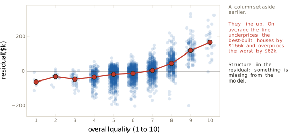
The deepest failure is visible in the residuals themselves. Figure 2.26 plots the residuals of Equation 2.19 against the quality rating, one of the columns set aside when living area was chosen. Averaged at each level of quality, the residuals rise with the rating. The line underprices the 26 best-built houses by $166 thousand on average and overprices the four houses rated lowest by $62 thousand, although four houses is a thin basis for the second figure. Structure in the residual means something is missing from the model, which is the lesson of Neptune in Section 1.1. What the line left behind is not noise. It is another column.
So one input is not enough, and the next section gives the line a second input and a third. Every computation of this section then has to be done again with many weights at once, and doing it shows that least squares is a projection.
Exercises
For each of the four families in Equation 2.1, count the parameters and state which of the other families it contains. Use the nesting to explain why the cubic fit in Figure 2.3 can never have a larger RSS on the same sales than the straight-line fit, and why that fact alone is no reason to prefer the cubic.
Classify each of the following as part of the true model or as something computed from the data, and give its meaning in words for the Ames problem: \(b\), \(\hat{w}\), \(\varepsilon_i\), \(\hat{y}_i\), \(r_i\), \(\bar{y}\), \(\mathrm{RSS}(\hat{b}, \hat{w})\). Then explain why \(r_i\) and \(\varepsilon_i\) are different quantities even for the sale on which both are defined, and say which of the two can be plotted.
Three sales have areas 100, 140 and 180 square metres and prices 150, 190 and 200 thousand dollars. Use Equation 2.18 to find \(\hat{w}\) and \(\hat{b}\). Compute the three residuals and check that they satisfy both equations of Equation 2.16. Then compute the RSS of the line, the RSS of the mean as a predictor, and \(R^2\) by Equation 2.20.
Gradient descent on the Ames bowl starts at \((\hat{b}, \hat{w}) = (110, 30)\) in the centred units of Equation 2.5, with \(\eta = 0.0001\). Using Equation 2.13 and Equation 2.6, together with \(n = 2{,}924\), \(\bar{y} = 180.42\), \(S_{uu} = 596.76\) and the bottom \(\hat{w} = 125.10\), compute the gradient at the start and the candidate after one step. Explain the signs of both partial derivatives by locating the start on Figure 2.12.
The centred bottom is \((\hat{b}, \hat{w}) = (180.4, 125.1)\) with \(\bar{x} = 138.8\) square metres. Convert it to everyday units and check the result against Equation 2.19. Then find the slope of the least-squares line if area were recorded in square feet instead of square metres, given that one square metre is 10.764 square feet, and state what happens to \(\hat{b}\), to the RSS and to \(R^2\).
Derive Equation 2.8 from Equation 2.4 written in centred units. Expand the square, use Equation 2.6 to remove the cross terms, and complete the square in each parameter. Deduce that the RSS has exactly one minimum, that the minimum value is \(S_{yy} - S_{uy}^2/S_{uu}\), and that \(R^2 = S_{uy}^2/(S_{uu}\,S_{yy})\) for the least-squares line.
Using Equation 2.14, Equation 2.13 and Equation 2.6, show that each step of gradient descent multiplies \(\hat{b} - \bar{y}\) by \(1 - 2n\eta\) and multiplies the distance of \(\hat{w}\) from its best value by \(1 - 2S_{uu}\eta\). With the Ames values of exercise 4, find how many steps are needed from \(\hat{w} = 30\) before \(\hat{w}\) is within 0.05 of 125.10, and compare the answer with the sixty steps of Figure 2.16. Then find the largest step size for which the walk does not move away from the bottom in either direction, and explain why it is smaller than the largest step size the cut along \(\hat{w}\) alone would tolerate.
Suppose living area is entered twice, as \(x\) in square metres and as \(10.764\,x\) in square feet, so that the hypothesis space is \(\hat{y} = \hat{b} + \hat{w}_1 x + \hat{w}_2 (10.764\,x)\). Show that every pair \((\hat{w}_1, \hat{w}_2)\) with \(\hat{w}_1 + 10.764\,\hat{w}_2 = 1.251\), together with \(\hat{b} = 6.78\), gives the same RSS as Equation 2.19. Explain what this means for the equations obtained by setting all three partial derivatives to zero, and connect the answer to the right-hand panel of Figure 2.18.
2.2 Multiple Regression and the Geometry of Least Squares
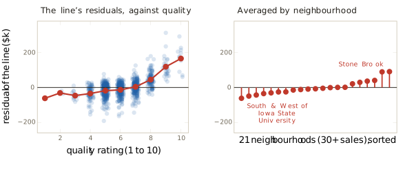
Section 2.1 fitted a straight line through living area and stopped at a diagnosis. The line explains about half of the variation in price, \(R^2 = 0.518\), and its residuals are not noise. Plotted against the quality rating, a column the line never read, they climb: the line overprices the worst-built houses by about $62 thousand on average and underprices the best-built by about $166 thousand (Figure 2.26). Averaged by neighbourhood they sort just as clearly. Sales in Stone Brook sit well above the line, and sales in the area south and west of Iowa State University sit below it. Figure 2.27 shows both. By the lesson of Neptune in Section 1.1, structure in the residual means that something is missing from the model, and here the missing things are named columns of the same file.
Practice reached the same conclusion long before any course on machine learning. A county assessor must put a value on every property in the county at each revaluation, far too many to inspect one at a time, and the values come from models fitted to recorded sales on recorded columns, with regression among the standard tools. Economists price a house feature by feature, asking what a bedroom, a garage or a better neighbourhood adds to the price when everything else about the house is held fixed. Rosen gave the economic theory of such hedonic prices in the Journal of Political Economy in 1974 (Rosen 1974), assuming that a good is valued as a bundle of characteristics, each with its own implicit price. The phrase everything else held fixed will turn out to be exactly what a weight means once a model has several inputs.
The problem of this section is therefore to predict a price from every column that matters, at once. Adding columns to the line looks like a small step, and it breaks three things that Section 2.1 relied on. The first is the notation. Written out term by term, a model with every recorded input of the Ames file, seventy-nine of them once the price and two identifiers are set aside, is a sum of eighty terms, and every statement about it would have to be made eighty times. The second is the solution. The closed form Equation 2.17 has one slope and no room for a second. The third is uniqueness. Section 2.1 showed that two inputs carrying the same information leave a whole line of equally good answers (Figure 2.18), and the Ames file contains such a pair for real. The section takes the three in order. It builds the language of vectors and matrices from the house data, uses it to show that least squares is a projection, derives the normal equations from that picture and from calculus, and then deals with the columns that break the method.
In the terms of Definition 1.16, the slot that moves is the hypothesis space. It grows from lines to flat surfaces. The loss is the residual sum of squares of Definition 2.3, unchanged, and the optimiser gains an exact form for any number of inputs.
Two inputs: a flat surface
With two inputs the model can still be drawn. Each sale is a point over its living area and its quality rating, at the height of its price, and the natural generalisation of a straight line is a flat surface through the cloud of points. The true model of Definition 2.2 extends in the obvious way.
Definition 2.10 (Multiple regression) Multiple regression is predicting a number from several recorded inputs at once. Its true model, for \(p\) inputs, asserts that \[ y_i \;=\; b + w_1\,x_{i1} + w_2\,x_{i2} + \cdots + w_p\,x_{ip} + \varepsilon_i , \qquad i = 1, \ldots, n , \tag{2.22}\] where \(x_{ij}\) is input \(j\) of sale \(i\), the intercept \(b\) and the weights \(w_1, \ldots, w_p\) are fixed numbers, the same for every sale, and the error term \(\varepsilon_i\) is everything about sale \(i\) that the model leaves out.
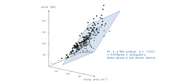
As in Section 2.1, the quantities of Equation 2.22 are the world’s and carry no hats. Note the change of notation from Section 2.1, where \(x_i\) was the area of sale \(i\). With several inputs a sale needs two indices, and \(x_{ij}\) is its input \(j\). Fitted by least squares to the 2,924 sales, with living area in square metres as input 1 and the quality rating as input 2, the model is
\[ \hat{y} \;=\; -113.1 \,+\, 0.676\,\text{area} \,+\, 32.8\,\text{quality} , \tag{2.23}\]
with prices in thousands of dollars. We call this fit 1. It explains \(R^2 = 0.751\) of the variation in price, against 0.518 for living area alone and 0.648 for quality alone. Figure 2.28 draws it among the sales.
A flat surface is hard to read directly, so we cut it. Holding quality at a fixed level turns Equation 2.23 into a straight line in area with slope 0.676, and changing the level moves that line up by 32.8 for each quality point without tilting it. The surface is therefore a family of parallel lines, one for each quality level, and Figure 2.29 draws them. Along the quality-6 line, a house 100 square metres larger is predicted to sell for $67.6 thousand more. The line of Section 2.1, fitted to area alone, is steeper than every one of them: alone, area’s weight was $1,251 per square metre, and with quality in the model it is $676.
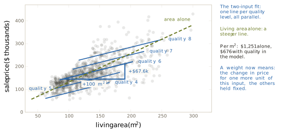
The two numbers measure different things, and the difference is the meaning of a weight in a model with several inputs. A weight \(\hat{w}_j\) is the change in the predicted price for one more unit of input \(j\), with the other inputs held fixed. Area’s weight fell because area and quality move together in Ames. Houses rated 4 average 107 square metres and houses rated 8 average 175. Fitted alone, the line in area crosses the quality lines of Figure 2.29, from the lower ones on the left to the upper ones on the right. Its slope therefore carries two effects. One is that of more floor space, and the other is the jump to a higher quality line that larger houses tend to make. The decomposition is exact. If \(\hat{\delta}\) is the slope of the least-squares line of quality on area, here 0.01754 quality points per square metre, then
\[ 1.251 \;=\; 0.6757 \;+\; 32.80 \times 0.01754 , \tag{2.24}\]
the slope alone is the slope with quality held fixed plus quality’s weight times the rate at which quality rises with area (exercise 8 proves the identity). The weights are printed here to four figures so that the sum checks. The value of \(\hat{\delta}\) is far below the 4 points per 68 square metres of the averages just quoted. Those averages read the relation the other way, area at a given quality, and for two columns that do not move in exact step the two slopes are not reciprocals of each other. A weight’s meaning therefore depends on which other columns are in the model, and adding a column changes the question each weight answers. It does not turn the weight into a causal effect: 0.676 describes how price varies with area among Ames houses of equal quality, and says nothing on its own about what an extension would do to one house.
Least squares had several unknowns from the start. Legendre’s appendix of 1805 set out the method for a system of equations in several unknowns (Legendre 1805), and Gauss in 1809 applied it to the elements of a planetary orbit (Gauss 1809). What Equation 2.22 lacks is a way to write it once for any \(p\), and that is a matter of language.
Scalars, vectors and matrices
The language is linear algebra, and Section 1.4 named it among the foundations of machine learning for exactly this purpose: a model that takes several inputs at once. We build it from the house data, one object at a time. The running example is the house held back from every fit in Section 2.1: 133.8 square metres, quality 5, built in 1968, sold for $163.0 thousand.
Definition 2.11 (Scalar and vector) A scalar is a single number. A vector is an ordered list of numbers, written as a column. The number of its entries is its dimension, and a vector of dimension \(k\) has shape \(k \times 1\): \(k\) rows and one column.
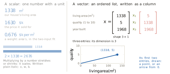
The living area of our house, 133.8 square metres, is a scalar, and so are its price and each weight of Equation 2.23. Multiplying a number by a scalar stretches it or shrinks it, which is where the name comes from. Scalars are set in plain italic: \(x\), \(w\), \(b\), \(n\), \(p\). The three recorded inputs of our house form a vector,
\[ \mathbf{x} \;=\; \begin{bmatrix} 133.8 \\ 5 \\ 1968 \end{bmatrix} , \]
set in bold, with entries \(x_1\), \(x_2\), \(x_3\), dimension 3 and shape \(3 \times 1\). The order carries meaning. Exchanging the first two entries describes a house of 5 square metres with a quality rating of 133.8, which is not our house and not a house at all. A vector of two entries can also be drawn, as a point of the plane or as an arrow from the origin to that point, and Figure 2.30 draws our house’s area and quality both ways. The arrow will matter.
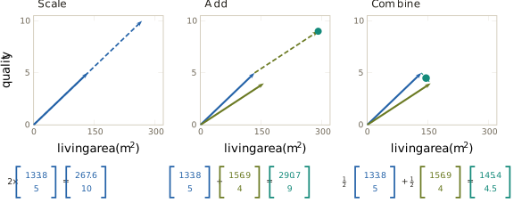
Two operations on vectors are needed, and both work entry by entry. A vector is multiplied by a scalar by multiplying every entry, so \(2 \times (133.8, 5) = (267.6, 10)\), and the arrow keeps its direction and doubles its length. Two vectors of the same shape are added by adding their entries. Taking a second house of 156.9 square metres and quality 4, \((133.8, 5) + (156.9, 4) = (290.7, 9)\), and as arrows the second is placed with its tail at the tip of the first. Vectors of different shapes cannot be added, because no entry of one has a partner in the other.
Definition 2.12 (Linear combination) A linear combination of vectors \(\mathbf{v}_1, \ldots, \mathbf{v}_k\) of the same shape is a sum \(c_1\mathbf{v}_1 + \cdots + c_k\mathbf{v}_k\), each vector multiplied by a scalar.
Half of our house plus half of the other is \(\tfrac12(133.8, 5) + \tfrac12(156.9, 4) = (145.4, 4.5)\), the house exactly midway between them. Figure 2.31 draws the three operations.
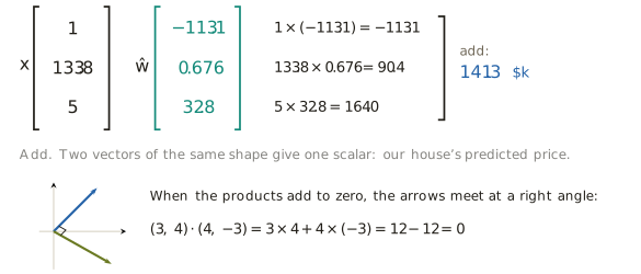
The weights of a fit are a vector too. Fit 1 has three numbers, and stacked they are \(\hat{\mathbf{w}} = (\hat{b}, \hat{w}_1, \hat{w}_2) = (-113.1, 0.676, 32.8)\), of shape \(3 \times 1\). Fit 1 reads only area and quality, so our house is described by two inputs. To give it the same shape as \(\hat{\mathbf{w}}\) we put a 1 in front: \(\mathbf{x} = (1, 133.8, 5)\). The intercept multiplies no input and is added once to every prediction, so its input is always 1. From here on every house vector carries this leading 1 as entry 0, and the intercept is weight 0, \(\hat{w}_0 = \hat{b}\). Pairing the entries of the two vectors, multiplying each pair and adding gives the prediction:
\[ 1 \times (-113.1) \;+\; 133.8 \times 0.676 \;+\; 5 \times 32.8 \;=\; -113.1 + 90.4 + 164.0 \;=\; 141.3 . \]
Definition 2.13 (Dot product) The dot product of two vectors of the same shape is the sum of the products of their corresponding entries: \[ \mathbf{x} \cdot \hat{\mathbf{w}} \;=\; \sum_{j=0}^{p} x_j\,\hat{w}_j . \tag{2.25}\] It takes two vectors and returns a scalar.
One prediction is a dot product, \(\hat{y} = \mathbf{x} \cdot \hat{\mathbf{w}}\), and Equation 2.25 holds whether \(p\) is two or eighty. That is the first of the three difficulties settled: the model is written once, for any number of inputs. Our house is predicted at $141.3 thousand by fit 1. Adding year built as a third input and fitting again to all 2,924 sales gives four weights, \((-1{,}071.4,\ 0.724,\ 25.42,\ 0.5055)\), and with \(\mathbf{x} = (1, 133.8, 5, 1968)\) the four products are \(-1{,}071.4\), \(96.9\), \(127.1\) and \(994.8\), so the prediction is $147.4 thousand, $15.6 thousand below the sale price. The large negative intercept is the price the fit assigns to a house with every input zero: no floor area, quality 0, built in year zero. No such house exists, and an intercept is not to be read on its own when zero is not a real value of the inputs.
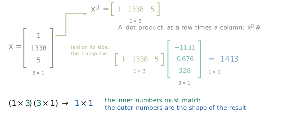
A compact notation for the dot product comes from turning a column on its side. The transpose of a column vector \(\mathbf{x}\), written \(\mathbf{x}^\top\), is the same entries laid out as a row, of shape \(1 \times 3\) when \(\mathbf{x}\) is \(3 \times 1\). A row times a column is computed by walking along the row and down the column together, multiplying and adding, which is the dot product:
\[ \hat{y} \;=\; \mathbf{x}^\top \hat{\mathbf{w}} . \tag{2.26}\]
Written with shapes, \((1 \times 3)(3 \times 1) \to 1 \times 1\). The inner numbers must match, since each entry of the row needs a partner in the column, and the outer numbers give the shape of the result. This shape rule checks every product in the rest of the section. Figure 2.33 draws it on our house.
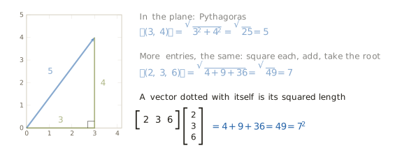
A vector has a length, and in the plane Pythagoras gives it. The arrow to \((3, 4)\) is the long side of a right triangle with sides 3 and 4, so its length is \(\sqrt{9 + 16} = 5\). With more entries the recipe is the same.
Definition 2.14 (Length) The length of a vector \(\mathbf{v}\) with entries \(v_1, \ldots, v_k\) is \[ \lVert \mathbf{v} \rVert \;=\; \sqrt{v_1^2 + \cdots + v_k^2} , \qquad\text{so that}\qquad \lVert \mathbf{v} \rVert^2 \;=\; \mathbf{v}^\top \mathbf{v} . \tag{2.27}\]
For \((2, 3, 6)\) the squares add to \(4 + 9 + 36 = 49\), and the length is 7. The middle of the recipe, squaring each entry and adding, is the vector dotted with itself, which is the second form of Equation 2.27. Figure 2.34 draws both cases.
Length explains why a zero dot product means a right angle, which Figure 2.32 showed for \((3, 4)\) and \((4, -3)\). Expanding the squared length of a sum entry by entry,
\[ \lVert \mathbf{u} + \mathbf{v} \rVert^2 \;=\; \sum_j (u_j + v_j)^2 \;=\; \lVert \mathbf{u} \rVert^2 + 2\,\mathbf{u}\cdot\mathbf{v} + \lVert \mathbf{v} \rVert^2 . \tag{2.28}\]
The arrows \(\mathbf{u}\) and \(\mathbf{v}\), placed tip to tail, form a triangle whose third side is \(\mathbf{u} + \mathbf{v}\). Its sides obey Pythagoras exactly when the middle term vanishes, and by the converse of Pythagoras the triangle then has a right angle at the corner where \(\mathbf{u}\) ends and \(\mathbf{v}\) begins. The angle at that corner and the angle between the two arrows drawn from one point add to two right angles, so when one is a right angle so is the other. Two vectors whose dot product is zero are called perpendicular, or orthogonal, and the word applies in any number of dimensions, where it can no longer be checked by eye.
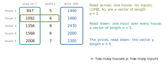
So far there has been one house. Ames has 2,924, and to keep the arithmetic visible we take five, chosen by a rule rather than by how well they fit: among the normal sales of single-family houses in 2008, the sale at the middle of each fifth of living area. Their areas are 84.7, 109.2, 135.6, 156.8 and 200.8 square metres, their quality ratings 5, 6, 8, 6 and 7, and their prices 144.0, 146.0, 247.0, 200.0 and 230.5 thousand dollars. The table can be read two ways (Figure 2.35). Read across a row, it gives one house: house 2’s inputs, \((109.2, 6)\), are a vector of dimension \(p = 2\), one entry per input, and \(p + 1\) entries with its leading 1. Read down a column, it gives one input over every house: the area column is a vector of dimension \(n = 5\), the number of houses. (The figure says “length” for the number of entries, which this book calls the dimension. Length in the sense of Definition 2.14 is a different thing.) The prices read down form the vector \(\mathbf{y}\), also of dimension \(n\). The letters are fixed from here on for the rest of the book: \(n\) counts observations and \(p\) counts inputs.
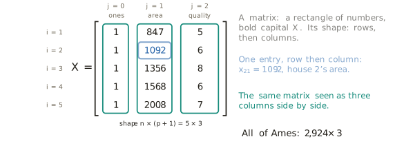
Definition 2.15 (Matrix) A matrix is a rectangle of numbers, set as a bold capital. A matrix with \(r\) rows and \(k\) columns has shape \(r \times k\), and its entry in row \(i\) and column \(j\) is written with the row first. The design matrix \(\mathbf{X}\) of a regression has one row per observation and one column per input, preceded by a column of ones, so that its shape is \(n \times (p + 1)\) and its entry \(x_{ij}\) is input \(j\) of observation \(i\), with \(x_{i0} = 1\). Its transpose \(\mathbf{X}^\top\) has the rows of \(\mathbf{X}\) as its columns, and shape \((p + 1) \times n\).
For the five houses, \(\mathbf{X}\) is \(5 \times 3\), and \(x_{21} = 109.2\) is house 2’s input 1, its area. Columns are counted from zero, so the ones column is column 0. For all of Ames the same two inputs give a matrix of shape \(2{,}924 \times 3\). Row \(i\) of \(\mathbf{X}\), stood upright, is the vector \(\mathbf{x}_i\) of house \(i\) with its leading 1. Read down, the same matrix is three columns side by side, and we write \(\mathbf{c}_j\) for column \(j\): here \(\mathbf{c}_0 = \mathbf{1}\), the column of ones, \(\mathbf{c}_1\) the areas and \(\mathbf{c}_2\) the quality ratings. Figure 2.36 shows both readings.
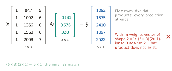
Every prediction can now be computed at once. Dotting each row of \(\mathbf{X}\) with \(\hat{\mathbf{w}}\) gives one prediction per house, and the \(n\) predictions stacked form a vector. This is the product of a matrix and a vector:
\[ \hat{\mathbf{y}} \;=\; \mathbf{X}\hat{\mathbf{w}}, \qquad \hat{y}_i \;=\; \mathbf{x}_i^\top \hat{\mathbf{w}} \;=\; \sum_{j=0}^{p} x_{ij}\,\hat{w}_j , \tag{2.29}\]
with shapes \((n \times (p+1))((p+1) \times 1) \to n \times 1\). For house 1, \(1 \times (-113.1) + 84.7 \times 0.676 + 5 \times 32.8 = 108.2\), and the five predictions under fit 1 are 108.2, 157.5, 241.0, 189.7 and 252.2 (Figure 2.37). The shape rule catches a mistake before any arithmetic: with a weight vector of shape \(2 \times 1\) the product would be \((5 \times 3)(2 \times 1)\), the inner numbers differ, and the product does not exist.
The same sum can be taken in the other order. Collecting the terms of Equation 2.29 by \(j\) instead of by \(i\),
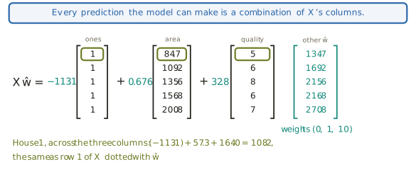
\[ \mathbf{X}\hat{\mathbf{w}} \;=\; \hat{w}_0\,\mathbf{c}_0 + \hat{w}_1\,\mathbf{c}_1 + \cdots + \hat{w}_p\,\mathbf{c}_p , \tag{2.30}\]
since entry \(i\) of the right-hand side is \(\sum_j \hat{w}_j\,x_{ij}\), which is \(\hat{y}_i\). For fit 1 this reads \(-113.1 \times \mathbf{1} + 0.676 \times (\text{area column}) + 32.8 \times (\text{quality column})\), and on house 1 it gives \(-113.1 + 57.3 + 164.0 = 108.2\), the number the row gave. Equation 2.30 is a linear combination in the sense of Definition 2.12, with the weights as its scalars. Another choice of weights, say \((0, 1, 10)\), is another combination, and gives another set of five predictions: 134.7, 169.2, 215.6, 216.8 and 270.8. The conclusion is the most important step on the way to the geometry. Every prediction the model can make, for any choice of weights, is a linear combination of the columns of \(\mathbf{X}\), and nothing else is available to it.
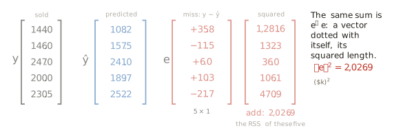
The residuals follow in the same way. Definition 1.3 wrote the residual of observation \(i\) as \(r_i\), and from here on we write it \(e_i\). Collected into a vector, the residuals become the residual vector,
\[ \mathbf{e} \;=\; \mathbf{y} - \mathbf{X}\hat{\mathbf{w}} , \tag{2.31}\]
of shape \(n \times 1\), with entries \(e_i = y_i - \hat{y}_i\). For the five houses under fit 1 the printed entries are \(+35.8\), \(-11.5\), \(+6.0\), \(+10.3\) and \(-21.7\). The residual sum of squares of Definition 2.3 is the sum of their squares, and by Equation 2.27 that is the squared length of \(\mathbf{e}\):
\[ \mathrm{RSS}(\hat{\mathbf{w}}) \;=\; \sum_{i=1}^{n} e_i^2 \;=\; \lVert \mathbf{y} - \mathbf{X}\hat{\mathbf{w}} \rVert^2 \;=\; (\mathbf{y} - \mathbf{X}\hat{\mathbf{w}})^\top(\mathbf{y} - \mathbf{X}\hat{\mathbf{w}}) . \tag{2.32}\]
The squares of the five printed residuals add to 2,026.9, in units of thousands of dollars squared. Computed from the fit’s unrounded weights, rather than from the three-figure weights printed here, the RSS of these five houses is 2,031.8. The score that Section 2.1 minimised, written for any number of inputs, is one squared length, and least squares means making the residual vector as short as possible.
Every piece of Equation 2.22 now has a single symbol, and the model takes one line. The true model and its estimate are
\[ \mathbf{y} \;=\; \mathbf{X}\mathbf{w} + \boldsymbol{\varepsilon}, \qquad\qquad \hat{\mathbf{y}} \;=\; \mathbf{X}\hat{\mathbf{w}} , \tag{2.33}\]
for one input or for eighty. Table 2.1 fixes the notation for the rest of the book. Italic lower case is a scalar, bold lower case a vector, bold capital a matrix, and a hat marks an estimate. Vectors are columns unless transposed.
| Symbol | Kind | Shape | What it is |
|---|---|---|---|
| \(n\) | scalar | one number | the number of observations (2,924 sales in Ames) |
| \(p\) | scalar | one number | the number of inputs |
| \(x_{ij}\) | scalar | one number | input \(j\) of observation \(i\), with \(x_{i0} = 1\) |
| \(\mathbf{x}_i\) | vector | \((p + 1) \times 1\) | observation \(i\)’s inputs, with its leading 1 |
| \(\mathbf{y}\) | vector | \(n \times 1\) | every recorded answer, here every price |
| \(\mathbf{w}\), \(\hat{\mathbf{w}}\) | vector | \((p + 1) \times 1\) | the true weights, never known, and their estimate |
| \(\boldsymbol{\varepsilon}\) | vector | \(n \times 1\) | everything the true model leaves out, never known |
| \(\hat{\mathbf{y}}\), \(\mathbf{e}\) | vector | \(n \times 1\) | every prediction, and every residual \(\mathbf{y} - \hat{\mathbf{y}}\) |
| \(\mathbf{X}\) | matrix | \(n \times (p + 1)\) | every input of every observation, a column of ones first |
Least squares as a projection
The language computes every prediction for any weights. The question left is which weights give the best predictions, and reading the table down turns that question into a picture.
To draw it we keep three of the five houses, the first, third and fifth, and two columns, the ones and living area, with area in hundreds of square metres and prices in hundreds of thousands of dollars. The three houses are renumbered 1 to 3, so that house 2 of this picture is house 3 of Figure 2.35. The familiar picture plots each house as a point, area against price, and fits a line through the three points. The second picture makes each house an axis. With three houses the space has three axes, and three numbers, one per house, are one point of it, or one arrow from the origin. Each column of \(\mathbf{X}\) then becomes one arrow: the ones column is the arrow to \((1, 1, 1)\), the area column the arrow to \((0.847, 1.356, 2.008)\). The prices are the arrow \(\mathbf{y} = (1.44, 2.47, 2.305)\). A house that was a point in the first picture is, in the second, one coordinate of every arrow (Figure 2.40). With \(n\) houses the same construction gives a space of \(n\) dimensions, which cannot be drawn and does not need to be, since every statement below is made with dot products and lengths, and they work in any number of dimensions.
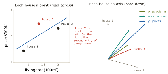
By Equation 2.30, every prediction \(\mathbf{X}\hat{\mathbf{w}}\) is a combination of the column arrows. In the house space, the combinations of two arrows fill a flat surface through the origin, and every prediction the model can make lies on it.
Definition 2.16 (Span) The span of a set of vectors is the set of all their linear combinations. The span of the columns of \(\mathbf{X}\) is the set of every prediction \(\mathbf{X}\hat{\mathbf{w}}\) the model can make.
The prices \(\mathbf{y}\) lie off the surface (Figure 2.41), and that is a fact about the data, not a defect of the drawing: \(\mathbf{y}\) would lie on it only if some line passed exactly through all three houses of Figure 2.40, and none does. This surface is not the surface of Figure 2.28. There each axis was an input and each point a house. Here each axis is a house, and each point is a whole vector of predictions.
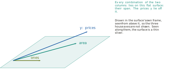
Least squares now has a geometric statement. Each candidate \(\hat{\mathbf{w}}\) is a point \(\mathbf{X}\hat{\mathbf{w}}\) of the span, and by Equation 2.32 its distance from \(\mathbf{y}\) is \(\lVert \mathbf{y} - \mathbf{X}\hat{\mathbf{w}} \rVert = \sqrt{\mathrm{RSS}}\). Minimising the RSS is finding the point of the span closest to \(\mathbf{y}\). Figure 2.42 marks two candidates. The weights \((-0.96, 1.34)\) give predictions at distance 2.13 from \(\mathbf{y}\), and the weights \((1.85, 0)\), a flat $185 thousand for every house whatever its area, give predictions at distance 0.87. The closest point of all lies straight below \(\mathbf{y}\), at distance 0.530. These distances are computed, not measured from the page: a perspective drawing of three dimensions shortens some lengths more than others, and in the figure the longer of the two dashed lines looks the shorter. It is the shadow that \(\mathbf{y}\) would cast on the surface with the light directly overhead, and at the shadow the residual vector stands at a right angle to the surface. The picture claims that this right angle is what makes the shadow closest, and the claim can be proved.
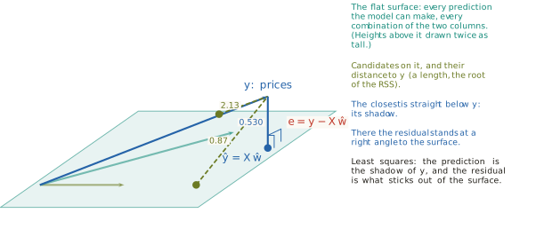
Suppose \(\hat{\mathbf{w}}\) is a candidate whose residual \(\mathbf{e} = \mathbf{y} - \mathbf{X}\hat{\mathbf{w}}\) is orthogonal to every column, \(\mathbf{c}_j \cdot \mathbf{e} = 0\) for \(j = 0, \ldots, p\). Take any other candidate \(\hat{\mathbf{w}}'\) and write \(\mathbf{d} = \hat{\mathbf{w}} - \hat{\mathbf{w}}'\). Its residual is
\[ \mathbf{y} - \mathbf{X}\hat{\mathbf{w}}' \;=\; \mathbf{e} + \mathbf{X}\mathbf{d} . \]
By Equation 2.30, \(\mathbf{X}\mathbf{d} = \sum_j d_j\,\mathbf{c}_j\), so its dot product with \(\mathbf{e}\) is \(\sum_j d_j\,(\mathbf{c}_j \cdot \mathbf{e}) = 0\). The two pieces are orthogonal, and Equation 2.28 gives
\[ \lVert \mathbf{y} - \mathbf{X}\hat{\mathbf{w}}' \rVert^2 \;=\; \lVert \mathbf{e} \rVert^2 + \lVert \mathbf{X}\mathbf{d} \rVert^2 \;\geq\; \lVert \mathbf{e} \rVert^2 . \tag{2.34}\]
No candidate has a smaller RSS than \(\hat{\mathbf{w}}\), and a candidate with the same RSS has \(\mathbf{X}\mathbf{d} = \mathbf{0}\) and therefore the same predictions. The argument shows that a candidate with an orthogonal residual is the best. That such a candidate always exists, for any \(\mathbf{X}\) and \(\mathbf{y}\), is a standard result of linear algebra, which this book uses without proof. The prediction \(\mathbf{X}\hat{\mathbf{w}}\) is the orthogonal projection of \(\mathbf{y}\) onto the span of the columns: the point of the span whose difference from \(\mathbf{y}\) is orthogonal to the span. This is the second promise printed under linear algebra in Section 1.4: least squares is a projection.
The condition is a set of equations, one per column. The dot products \(\mathbf{c}_j \cdot \mathbf{e}\), stacked, are the entries of \(\mathbf{X}^\top\mathbf{e}\), since the rows of \(\mathbf{X}^\top\) are the columns of \(\mathbf{X}\):
\[ \mathbf{X}^\top(\mathbf{y} - \mathbf{X}\hat{\mathbf{w}}) \;=\; \mathbf{0} , \tag{2.35}\]
with shapes \(((p+1) \times n)(n \times 1) \to (p+1) \times 1\): one equation per column. To write it without the bracket we need the product of two matrices.
Definition 2.17 (Matrix product) The product \(\mathbf{A}\mathbf{B}\) of an \(r \times k\) matrix \(\mathbf{A}\) and a \(k \times m\) matrix \(\mathbf{B}\) is the \(r \times m\) matrix whose entry in row \(i\) and column \(j\) is row \(i\) of \(\mathbf{A}\) dotted with column \(j\) of \(\mathbf{B}\). By the shape rule, the product exists only when the inner numbers agree: \((r \times k)(k \times m) \to r \times m\).
The matrix-vector product of Equation 2.29 is the case \(m = 1\). Order matters: \(\mathbf{A}\mathbf{B}\) can exist when \(\mathbf{B}\mathbf{A}\) does not, and even when both exist they generally differ. Matrix products distribute over sums as products of numbers do, \(\mathbf{A}(\mathbf{u} - \mathbf{v}) = \mathbf{A}\mathbf{u} - \mathbf{A}\mathbf{v}\), and multiplying out Equation 2.35 gives the central equations of the section.
Definition 2.18 (Normal equations) The normal equations of least squares are \[ \mathbf{X}^\top\mathbf{X}\,\hat{\mathbf{w}} \;=\; \mathbf{X}^\top\mathbf{y} . \tag{2.36}\] They state that the residual is orthogonal to every column of \(\mathbf{X}\).
The name is apt, since normal is the geometer’s word for perpendicular. The matrix \(\mathbf{X}^\top\mathbf{X}\) has shape \((p + 1) \times (p + 1)\), and its entry in row \(j\) and column \(k\) is \(\mathbf{c}_j \cdot \mathbf{c}_k\), one column dotted with another. Entry \(j\) of \(\mathbf{X}^\top\mathbf{y}\) is \(\mathbf{c}_j \cdot \mathbf{y}\). Equation 2.36 is the second difficulty settled: one formula for any number of inputs. Figure 2.43 marks the two right angles in the house space.
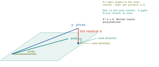
For the three houses of the picture the projection can be checked directly. The normal equations give \(\hat{\mathbf{w}} = (1.090, 0.699)\), the prediction \(\hat{\mathbf{y}} = (1.682, 2.038, 2.494)\) and the residual \(\mathbf{e} = (-0.242, 0.432, -0.189)\). Its dot product with the ones column is \(-0.242 + 0.432 - 0.189 = 0.001\), and with the area column \(0.847 \times (-0.242) + 1.356 \times 0.432 + 2.008 \times (-0.189) = 0.001\), both zero to the rounding of the printed digits, and its length is 0.530. The candidate \(\hat{\mathbf{w}}' = (0.248, 1.299)\) has a residual whose dot product with the ones column is zero and with the area column is \(-0.41\). It fails one of the equations, and by Equation 2.34 it is further from \(\mathbf{y}\): its distance is 0.724. A candidate is the least-squares answer only if every dot product is zero.
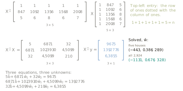
For the five houses with both inputs, Figure 2.44 computes every entry. The top-left entry of \(\mathbf{X}^\top\mathbf{X}\) is the ones column dotted with itself, \(1 + 1 + 1 + 1 + 1 = 5 = n\). The entries beside it are the sums of the areas, 687.1, and of the quality ratings, 32. The bottom-right entry is the sum of the squared ratings, \(25 + 36 + 64 + 36 + 49 = 210\). Written out, Equation 2.36 is three equations in three unknowns,
\[ \begin{aligned} 5\,\hat{b} \;+\; 687.1\,\hat{w}_1 \;+\; 32\,\hat{w}_2 &\;=\; 967.5, \\ 687.1\,\hat{b} \;+\; 102{,}393.0\,\hat{w}_1 \;+\; 4{,}509.9\,\hat{w}_2 &\;=\; 139{,}277.6, \\ 32\,\hat{b} \;+\; 4{,}509.9\,\hat{w}_1 \;+\; 210\,\hat{w}_2 &\;=\; 6{,}385.5, \end{aligned} \tag{2.37}\]
of the kind solved at school by elimination, and their solution is \(\hat{\mathbf{w}} = (-44.3, 0.386, 28.9)\). The same equations built from all 2,924 sales give fit 1, \((-113.1, 0.676, 32.8)\). Five houses give a rough estimate, and the full data give the fit. On the five houses alone, the five-house solution scores an RSS of 953.7 against fit 1’s 2,031.8, as it must, since it is the best for those five and for no others.
Legendre had already reduced least squares to such linear equations and left them to the ordinary methods of solution (Legendre 1805). Gauss solved them by elimination (Gauss 1809) and set out a systematic scheme for it in a memoir of 1810 on the orbit of the asteroid Pallas (Grcar 2011). To write their solution in one line, as Section 2.1 wrote the slope, two more objects are needed.
Definition 2.19 (Identity and inverse) The identity matrix \(\mathbf{I}\) is the square matrix with ones on its diagonal and zeros elsewhere. It changes nothing: \(\mathbf{I}\mathbf{v} = \mathbf{v}\) for every vector of matching shape. The inverse of a square matrix \(\mathbf{A}\), when it exists, is the matrix \(\mathbf{A}^{-1}\) with \(\mathbf{A}^{-1}\mathbf{A} = \mathbf{A}\mathbf{A}^{-1} = \mathbf{I}\).
For \(\mathbf{A} = \begin{bmatrix} 2 & 1 \\ 1 & 1 \end{bmatrix}\) the inverse is \(\mathbf{A}^{-1} = \begin{bmatrix} 1 & -1 \\ -1 & 2 \end{bmatrix}\). By Definition 2.17 the top-left entry of \(\mathbf{A}^{-1}\mathbf{A}\) is \(1 \times 2 + (-1) \times 1 = 1\), and the other three entries come out as the identity requires. With a single number the inverse is division: \(\tfrac14 \times 4 = 1\). Read this way, \(\mathbf{X}^\top\mathbf{X}\) is a matrix that takes \(\hat{\mathbf{w}}\) to \(\mathbf{X}^\top\mathbf{y}\), as multiplying by 4 takes a quarter to one, and its inverse undoes it. Multiplying both sides of Equation 2.36 by \((\mathbf{X}^\top\mathbf{X})^{-1}\) gives the least-squares solution,
\[ \hat{\mathbf{w}} \;=\; (\mathbf{X}^\top\mathbf{X})^{-1}\,\mathbf{X}^\top\mathbf{y} , \tag{2.38}\]
for any number of inputs, whenever the inverse exists. When it does not is the subject of the last part of this section. In practice the system Equation 2.36 is solved by elimination without forming the inverse, which is faster and more accurate, and the cost and accuracy of that work are taken up in Section 2.4.
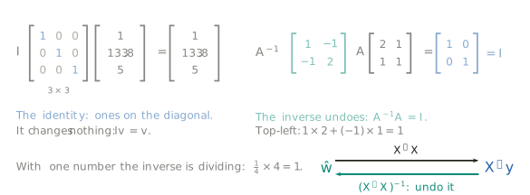
Matrices arose as shorthand for such systems. Cayley set out their algebra, including the product and the inverse, in A Memoir on the Theory of Matrices, published in the Philosophical Transactions of the Royal Society in 1858 (Cayley 1858). He described a matrix as a convenient notation for a set of linear equations.
The normal equations also follow from calculus, by the route of Section 2.1, and the two routes must agree. Moving weight \(\hat{w}_j\) by \(h\) changes each residual \(e_i\) to \(e_i - h\,x_{ij}\), so its square changes by \(-2h\,x_{ij}\,e_i + h^2 x_{ij}^2\). Dividing by \(h\) and letting \(h\) go to zero leaves \(-2\,x_{ij}\,e_i\), and adding over the observations gives
\[ \frac{\partial\,\mathrm{RSS}}{\partial \hat{w}_j} \;=\; -2 \sum_{i=1}^{n} x_{ij}\,e_i \;=\; -2\,\mathbf{c}_j \cdot \mathbf{e}, \qquad\text{so}\qquad \nabla \mathrm{RSS} \;=\; -2\,\mathbf{X}^\top\mathbf{e} . \tag{2.39}\]
This is Equation 2.13 for any number of inputs. The gradient is zero exactly when \(\mathbf{X}^\top\mathbf{e} = \mathbf{0}\), which is Equation 2.35. The calculus route says that every minimiser satisfies the normal equations, and the geometric route says that every solution of them is a minimiser, so the two together identify the least-squares answers with the solutions of Equation 2.36.
With one input the general result becomes the formula of Section 2.1. Measure area from the average house and in hundreds of square metres, as in Equation 2.5, so that \(\mathbf{X}\) has two columns, the ones and \(\mathbf{u}\). Then
\[ \mathbf{X}^\top\mathbf{X} \;=\; \begin{bmatrix} n & \sum_i u_i \\ \sum_i u_i & \sum_i u_i^2 \end{bmatrix} \;=\; \begin{bmatrix} n & 0 \\ 0 & S_{uu} \end{bmatrix}, \qquad \mathbf{X}^\top\mathbf{y} \;=\; \begin{bmatrix} \sum_i y_i \\ S_{uy} \end{bmatrix} , \tag{2.40}\]
where the zeros are Equation 2.6. The two normal equations are \(n\hat{b} = \sum_i y_i\) and \(S_{uu}\,\hat{w} = S_{uy}\), which are Equation 2.16 and give Equation 2.17: \(\hat{b} = \bar{y}\) and \(\hat{w} = 125.1\) thousand dollars per extra hundred square metres, the line of Section 2.1. The slope formula now reads differently. Its numerator \(\sum_i u_i y_i\) is the dot product \(\mathbf{u}^\top\mathbf{y}\), its denominator \(\sum_i u_i^2\) is \(\mathbf{u}^\top\mathbf{u}\), and dividing is multiplying by the inverse of a \(1 \times 1\) matrix:
\[ \hat{w} \;=\; \frac{\sum_i u_i\,y_i}{\sum_i u_i^2} \;=\; (\mathbf{u}^\top\mathbf{u})^{-1}\,\mathbf{u}^\top\mathbf{y} , \]
which is Equation 2.38 with one column. The formula of Section 2.1 was the normal equations from the start (Figure 2.46).
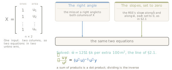
Columns that need work
Equation 2.38 accepts any columns of numbers, and not every column arrives as one. The neighbourhood of a sale is a name, such as North Ames, Stone Brook or Briardale, and a name cannot be multiplied by a weight.
Definition 2.20 (Indicator column) An indicator column for a category is a column that holds 1 for every observation in that category and 0 for every other.
Ames has 28 neighbourhoods, and one indicator per name gives 28 columns. The weight on an indicator is added to the prediction only for sales in that neighbourhood, so each name moves the whole surface up or down without changing its slopes (Figure 2.47). Turning a name into numbers is not yet machine learning. It is the preparation of data, which Section 1.3 placed among the stages of data science.
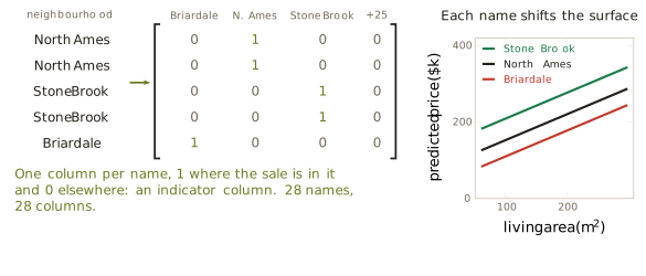
Placed beside the ones column, the indicators contain a trap. Every sale is in exactly one neighbourhood, so in every row the 28 indicators add to 1, and the sum of the indicator columns is the ones column. One column is a combination of the others. Suppose a weight vector gives some set of predictions. Raising the intercept by 50 and lowering every neighbourhood’s weight by 50 changes no prediction, since every row gains 50 from the intercept and loses 50 from its one indicator, and the RSS is unchanged. Least squares then has no unique answer. With area, quality, year built and all 28 indicators, \(\mathbf{X}\) has 32 columns, but as the next part makes precise, only 31 of them are genuinely different.
The remedy is to drop one indicator. Its category becomes the reference, and the weight of every other category measures its shift from the reference. Here the reference is North Ames, the commonest neighbourhood with 443 sales. With area, quality and year built held fixed, a house in Briardale is predicted at $42.7 thousand less than a comparable house in North Ames, and a house in Stone Brook at $56.3 thousand more (Figure 2.48). The alternative remedy keeps every indicator and drops the ones column, so that each name carries its own level. Suits set out the difficulty and both remedies in Use of Dummy Variables in Regression Equations, published in the Journal of the American Statistical Association in 1957 (Suits 1957). The problem is known as the dummy-variable trap, dummy variable being the econometric name for an indicator column.
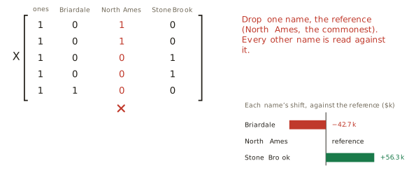
A second difficulty concerns units. With year built added, the fitted weights are 0.724 thousand dollars per square metre, 25.4 per quality point and 0.506 per year. Their sizes cannot be compared, since each carries the unit of its own column, and nothing follows from quality’s weight being thirty-five times area’s.
Definition 2.21 (Standardising) To standardise a column is to subtract its mean and divide by its standard deviation, so that entry \(i\) of input \(j\) becomes \[ z_{ij} \;=\; \frac{x_{ij} - m_j}{s_j} , \tag{2.41}\] where \(m_j\) and \(s_j\) are the mean and standard deviation of column \(j\) over the \(n\) observations, the standard deviation dividing by \(n\). One unit of a standardised column is one standard deviation of the original.
The standard deviations here are 45.18 square metres of living area, 1.403 quality points and 30.24 years. Refitted on standardised columns, the weights are 32.7, 35.7 and 15.3 thousand dollars per standard deviation. Measured per typical difference between houses, and with the other columns held fixed, area and quality move the price about equally and year built about half as much. The raw weights are recovered by dividing each by its column’s standard deviation: \(32.7 / 45.18 = 0.724\), \(35.7 / 1.403 = 25.4\) and \(15.3 / 30.24 = 0.506\).
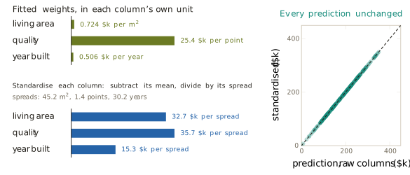
Every prediction is unchanged by standardising (Figure 2.49), and the projection explains why. By Equation 2.41 each raw column is \(\mathbf{c}_j = m_j\,\mathbf{1} + s_j\,\mathbf{z}_j\), a combination of the ones column and the standardised column, and each standardised column is in turn a combination of the ones column and the raw one. Every combination of one set is a combination of the other, so the two sets of columns have the same span. The projection of \(\mathbf{y}\) onto that span is the same point, and the predictions are the same numbers. Only the weights that reach the point change. Standardising matters again when the weights are found step by step rather than by solving, which is part of Section 2.4.
When the answer is not unique
The third difficulty is the one Section 2.1 met with area entered twice. Ames contains a repetition that nobody had to create. The file records first-floor area, second-floor area and low-quality finished area, and living area is exactly their sum in every one of the 2,924 sales (Figure 2.50). A model given the ones column and all four area columns has five columns, of which only four are genuinely different, since the fifth is built from three of the others.
Definition 2.22 (Rank) The rank of a matrix is the largest number of its columns that can be chosen so that none is a linear combination of the others. Going through the columns in order and keeping each one that is not a combination of those already kept, the number kept is the rank. A matrix has full column rank when its rank equals its number of columns.
The repeated-area matrix has rank 4 of 5, and the neighbourhood matrix with all 28 indicators rank 31 of 32. A column that repeats the others means some combination of the columns with weights not all zero is the zero vector, \(\mathbf{X}\mathbf{v} = \mathbf{0}\) with \(\mathbf{v} \neq \mathbf{0}\). The two statements say the same thing. If one column is a combination of the others, moving it to the other side of the equation gives such a \(\mathbf{v}\). If such a \(\mathbf{v}\) exists, any column whose entry of \(\mathbf{v}\) is not zero can be solved for in terms of the rest. For the area identity, \(\mathbf{v}\) takes \(+1\) on each floor column and \(-1\) on living area. Then \(\hat{\mathbf{w}}\) and \(\hat{\mathbf{w}} + t\,\mathbf{v}\) give the same predictions for every \(t\), and the RSS has a line of equally good bottoms, the trough of Figure 2.18 found in real data.
The formula fails with it. If \(\mathbf{X}\mathbf{v} = \mathbf{0}\) then \(\mathbf{X}^\top\mathbf{X}\mathbf{v} = \mathbf{0}\), so \(\mathbf{X}^\top\mathbf{X}\) sends a nonzero vector to zero. No matrix can undo that, since an inverse would have to send \(\mathbf{0}\) back to \(\mathbf{v}\), and \((\mathbf{X}^\top\mathbf{X})^{-1}\) does not exist. It is the matrix form of dividing by zero. The converse holds too. If \(\mathbf{X}^\top\mathbf{X}\mathbf{v} = \mathbf{0}\) for some \(\mathbf{v}\), then, writing the dot product of \(\mathbf{v}\) with it column by column,
\[ 0 \;=\; \mathbf{v} \cdot (\mathbf{X}^\top\mathbf{X}\mathbf{v}) \;=\; \sum_j v_j\,(\mathbf{c}_j \cdot \mathbf{X}\mathbf{v}) \;=\; (\mathbf{X}\mathbf{v}) \cdot (\mathbf{X}\mathbf{v}) \;=\; \lVert \mathbf{X}\mathbf{v} \rVert^2 , \tag{2.42}\]
so \(\mathbf{X}\mathbf{v} = \mathbf{0}\). A standard result of linear algebra, which this book uses without proof, says that a square matrix has an inverse exactly when the only vector it sends to zero is the zero vector. Together these give the condition for Equation 2.38: \((\mathbf{X}^\top\mathbf{X})^{-1}\) exists exactly when \(\mathbf{X}\) has full column rank. The projection \(\hat{\mathbf{y}}\) exists and is unique either way, since Equation 2.34 makes the closest point unique. What fails is only the uniqueness of the weights that reach it.
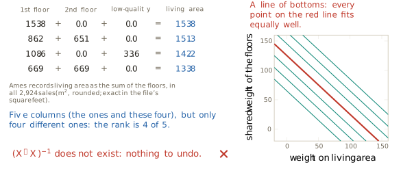
Exact repetition is easy to detect, because the rank says so. Near repetition is harder and in practice more common. The number of cars a garage holds and its floor area move together closely, with a correlation of 0.89 in Ames, where the correlation coefficient equals 1 when two columns rise in perfect step along a line. The matrix with both columns has full rank, and the weights exist and are unique, but they are not reliable. To see this, we drew 200 random samples of 60 different sales each and fitted the price on the two garage columns, standardised, with prices and columns centred so that the intercept drops out. Figure 2.51 plots each sample’s pair of weights. The weights scatter along a line, about \(27.6 \pm 21.3\) for garage cars and \(26.4 \pm 23.9\) for garage area, where \(\pm\) is the standard deviation across the samples. In 39 of the 200 samples one of the two weights is negative, so that, with the other garage column held fixed, a bigger garage lowers the predicted price. That is not a fact about houses. The data cannot separate two columns that say almost the same thing, so the weights trade off along the trough while the predictions barely move.
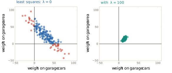
Both failures have a name.
Definition 2.23 (Well-posed problem) A problem is well-posed when its answer exists, is unique, and depends continuously on the data, so that a small change in the data produces only a small change in the answer. A problem that fails any of the three conditions is ill-posed.
Hadamard, in the Princeton University Bulletin in 1902, argued that a problem of mathematical physics should have a solution and only one, and that problems without this property do not correspond to physical situations (Hadamard 1902). The third condition, stability, is part of the standard statement of his definition today. Least squares with exactly repeated columns fails uniqueness, and with nearly repeated columns it fails stability.
The repair adds a cost for large weights. Instead of the RSS alone, minimise
\[ \mathrm{RSS}(\hat{\mathbf{w}}) + \lambda\,\lVert \hat{\mathbf{w}} \rVert^2 , \qquad \lambda > 0 . \tag{2.43}\]
The partial derivative of the penalty along \(\hat{w}_j\) is \(2\lambda\hat{w}_j\), so by Equation 2.39 the gradient is \(-2\,\mathbf{X}^\top\mathbf{e} + 2\lambda\hat{\mathbf{w}}\). Setting it to zero and using \(\hat{\mathbf{w}} = \mathbf{I}\hat{\mathbf{w}}\) gives \((\mathbf{X}^\top\mathbf{X} + \lambda\mathbf{I})\,\hat{\mathbf{w}} = \mathbf{X}^\top\mathbf{y}\). That this point is the minimiser, and not only a point where every slope is zero, follows as Equation 2.34 did. Expanding the score at another candidate \(\hat{\mathbf{w}} + \mathbf{d}\), the terms of first degree in \(\mathbf{d}\) come to \(-2\,\mathbf{d} \cdot (\mathbf{X}^\top\mathbf{e} - \lambda\hat{\mathbf{w}})\), which is zero at this point, and what remains adds \(\lVert \mathbf{X}\mathbf{d} \rVert^2 + \lambda\,\lVert \mathbf{d} \rVert^2\) to the score, a positive amount whenever \(\mathbf{d} \neq \mathbf{0}\).
Definition 2.24 (Tikhonov’s fix) Tikhonov’s fix replaces the least-squares solution by \[ \hat{\mathbf{w}}_\lambda \;=\; (\mathbf{X}^\top\mathbf{X} + \lambda\,\mathbf{I})^{-1}\,\mathbf{X}^\top\mathbf{y} , \qquad \lambda > 0 , \tag{2.44}\] the minimiser of Equation 2.43. The number \(\lambda\) sets the price of a large weight.
The inverse in Equation 2.44 always exists. Repeating the steps of Equation 2.42 for any vector \(\mathbf{v}\),
\[ \mathbf{v} \cdot \bigl( (\mathbf{X}^\top\mathbf{X} + \lambda\mathbf{I})\,\mathbf{v} \bigr) \;=\; \lVert \mathbf{X}\mathbf{v} \rVert^2 + \lambda\,\lVert \mathbf{v} \rVert^2 , \]
which is positive whenever \(\mathbf{v} \neq \mathbf{0}\), so the matrix sends no nonzero vector to zero. However the columns repeat, there is exactly one answer. Figure 2.52 shows what the penalty does to the score of one sample of 60. Least squares alone gives a long trough whose bottom sits at \((25.5, 36.0)\), wherever this particular sample happens to put it. With \(\lambda = 100\) the trough is lifted into a bowl with one clear bottom, at \((17.4, 17.6)\). Over all 200 samples (Figure 2.51), the spread of each weight falls from about 21 to 24 to about 3, and no weight changes sign. The price is visible too: the weights shrink, on average from about 27 to about 14. A steadier answer is bought by pulling the weights towards zero and away from what the data alone say. In this experiment the intercept was removed by centring and so was not penalised, which is the usual practice. How to choose \(\lambda\) is a question about data the fit has not seen, and Section 2.7 takes it up.
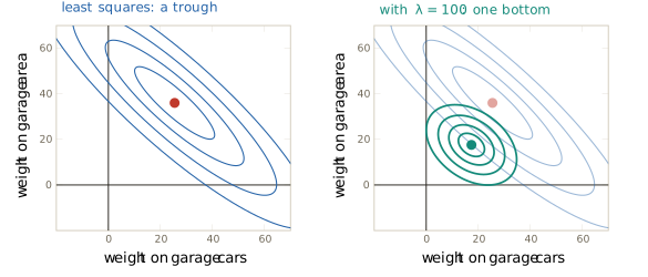
Tikhonov showed in 1943, in On the Stability of Inverse Problems in the Doklady of the Academy of Sciences of the Soviet Union, that an unstable inverse problem becomes stable when its answer is restricted to a suitably bounded set (Tikhonov 1943). In 1963 he gave the regularisation method, which adds a penalty on the size of the answer, in the Soviet Mathematics Doklady (Tikhonov 1963). Phillips had published the same idea independently a year earlier, for integral equations, in the Journal of the ACM (Phillips 1962), and the method is also called Tikhonov-Phillips regularisation. Its assumption is that, when the data cannot decide between answers, a smaller answer is preferable. The method is standard wherever a quantity is reconstructed from indirect and noisy measurements, as in image reconstruction, and it returns in Section 2.7 under the name statisticians gave it.
When the repetition is exact, a second way of choosing one answer exists. Enter living area twice, centred and in hundreds of square metres as in Equation 2.5. The intercept separates as in Equation 2.40. The score depends on the two area weights only through their sum, so every pair with \(\hat{w}_a + \hat{w}_b = 125.1\) is a bottom: the red line of Figure 2.53. Among them, the shortest in the sense of Definition 2.14 is the point nearest the origin, where a line from the origin meets the line of bottoms at a right angle. By symmetry it splits the slope evenly, \((62.6, 62.6)\).
Definition 2.25 (Pseudo-inverse) Among all the minimisers of the RSS, the one of smallest length, which is always unique (a standard result, stated here without proof), is written \(\mathbf{X}^{+}\mathbf{y}\), and \(\mathbf{X}^{+}\) is the pseudo-inverse of \(\mathbf{X}\). When \(\mathbf{X}\) has full column rank there is only one minimiser, and \(\mathbf{X}^{+}\mathbf{y}\) is Equation 2.38.
Tikhonov’s answers lead to the same point. In the doubled-area case \(\mathbf{X}^\top\mathbf{X}\) has all four entries equal to \(S_{uu}\), both entries of \(\mathbf{X}^\top\mathbf{y}\) equal \(S_{uy}\), and by symmetry Equation 2.44 gives equal weights \((t, t)\) with \(2S_{uu}t + \lambda t = S_{uy}\), so that
\[ t \;=\; \frac{S_{uy}}{2S_{uu} + \lambda} . \tag{2.45}\]
With \(S_{uu} = 596.76\) and \(S_{uy} = 74{,}655.9\), the values \(\lambda = 3{,}000\), \(1{,}000\), \(300\), \(100\) and \(10\) give \(t = 17.8\), \(34.0\), \(50.0\), \(57.7\) and \(62.0\). As \(\lambda\) shrinks to zero, \(t\) approaches \(S_{uy}/(2S_{uu}) = 62.6\), the shortest bottom. The same limit holds for any \(\mathbf{X}\), a result this book states without proof, and Tikhonov’s answer for a vanishing \(\lambda\) is the pseudo-inverse answer. Moore described a general reciprocal of any matrix in 1920, in the Bulletin of the American Mathematical Society (Moore 1920), and Penrose, unaware of Moore’s work, defined the same object by four algebraic conditions in the Proceedings of the Cambridge Philosophical Society in 1955 (Penrose 1955). It is what NumPy’s least-squares routine, built on the LAPACK library, returns when the columns repeat. Other software drops one of the repeated columns instead, as R’s linear-model function does. Its assumption is that, among answers the data cannot tell apart, the shortest is the one to report.
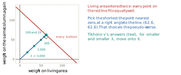
The third difficulty is now settled in both its forms. Exact repetition is a failure of rank and leaves the weights undetermined. Near repetition leaves them determined but unstable. Tikhonov’s fix repairs both at the price of a pull towards zero, and the pseudo-inverse chooses among exact ties. Why near repetition also makes the computation itself inaccurate, and why it slows a descent along the trough, is the subject of Section 2.4, and the spread of a weight across samples receives its name and its formula in Section 2.6.
Judging the fit
Definition 2.8 carries over unchanged to any number of inputs, provided \(\mathbf{X}\) contains the ones column. Figure 2.54 adds the columns one group at a time. Living area alone gives \(R^2 = 0.518\). Adding quality gives 0.751, the largest single step. Adding year built gives 0.775, and adding the neighbourhood, as 27 indicators against North Ames, gives 0.823, about four-fifths of the variation in price.
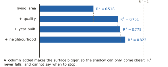
The bars only grow, and the projection shows that they must. Adding a column enlarges the span, and the old span lies inside the new one. The closest point of the larger set can be no further from \(\mathbf{y}\) than the closest point of the smaller, so the RSS cannot rise and \(R^2\) cannot fall, whatever the column holds, including a column of random numbers. \(R^2\) on the data used for fitting therefore cannot say when to stop adding columns. Choosing columns properly requires data the fit has not seen, which is the subject of Section 2.7.
The house held back from every fit gives a single-house view of the same ladder (Figure 2.55). It sold for $163.0 thousand. The line of Section 2.1 predicted $174.1 thousand. Fit 1 predicts $141.3 thousand, further off and on the other side, and the fit with year built and neighbourhood predicts $154.0 thousand. One house can move either way as columns are added, and a fit is judged over all the sales, which is what \(R^2\) measures. Over all the sales the change is plain. The residuals of Section 2.1 climbed steeply against quality. With quality, year built and neighbourhood in the model, the averages at the middle levels of quality lie close to zero, and the tilt is gone.
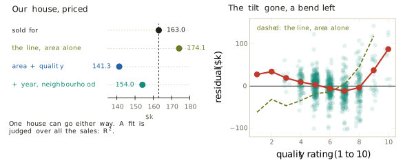
The three choices of Definition 1.16 have each moved or stayed (Figure 2.56). The hypothesis space is every flat surface over the inputs, one weight per input. The loss is the residual sum of squares, unchanged. The optimiser is the normal equations, solved once. On the modelling axis of Figure 2.7 the method sits where the line did: two things are our assumptions, the flat form and the choice of columns, and every weight comes from the data.
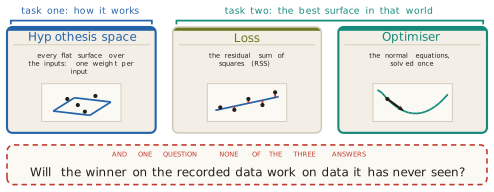
The residuals of the many-input fit have not finished speaking. Averaged at each level of quality (Figure 2.57), they lie within about $12 thousand of zero from level 4 to level 8, and they rise at both ends. The four houses rated 1 and the thirteen rated 2 sit about $28 thousand and $34 thousand above the surface, and the 26 best-built houses about $88 thousand above it. A flat surface cannot bend. A column holding the square of the quality rating would raise \(R^2\) from 0.823 to 0.847, and adding such a column keeps the model linear in its weights, so that everything in this section still applies. Section 2.3 takes up that move.
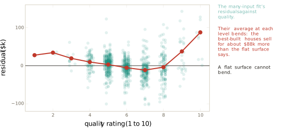
What the method assumes, and where it fails
The assumptions of Section 2.1 remain: only the price is in error, misses are judged by their squares, and the sales stand for the houses to be priced. Several inputs add assumptions of their own.
- The effects add. Each weight is the same at every level of the other inputs, so the effect of area is the same for a house of quality 4 as for one of quality 9. The parallel lines of Figure 2.29 are this assumption drawn.
- A rating entered as one number assumes equal steps. Entering quality as a single column says that the step from 4 to 5 is worth the same as the step from 9 to 10. The bend of Figure 2.57 is where this assumption fails.
- A weight is conditional on the other columns. It describes how the price varies with one input among houses equal in the others that are in the model. Adding or removing a column changes it, as Equation 2.24 shows, and no weight is by itself a causal effect.
- The columns must be genuinely different. With exact repetition the weights are not determined, and with near repetition they are determined but unstable from sample to sample, although the predictions may change little.
- A good fit on the recorded sales is not a good choice of columns. \(R^2\) never falls as columns are added, so it cannot decide which to keep.
Every result of the section rests on the model being linear in its weights, and nothing in it requires the columns to be the recorded inputs themselves. That is the opening for Section 2.3.
Exercises
The fit of Figure 2.54 with neighbourhood uses the ones column, area, quality, year built and 27 indicators, for the 2,924 sales. Give the shapes of \(\mathbf{X}\), \(\hat{\mathbf{w}}\), \(\mathbf{X}\hat{\mathbf{w}}\), \(\mathbf{e}\), \(\mathbf{X}^\top\mathbf{X}\), \(\mathbf{X}^\top\mathbf{y}\) and \(\mathbf{e}^\top\mathbf{e}\). Say which of \(\hat{\mathbf{w}}\mathbf{X}\), \(\mathbf{X}\mathbf{X}^\top\) and \(\mathbf{y}^\top\mathbf{X}\) exist, with their shapes. Then say what number each of these entries of \(\mathbf{X}^\top\mathbf{X}\) counts: the top-left entry, the entry in the row of the ones column and the column of the Briardale indicator, the diagonal entry of the Briardale indicator, and the entry for the Briardale and Stone Brook indicators.
For the three houses of Figure 2.40, \(\mathbf{c}_1 = (0.847, 1.356, 2.008)\) and \(\mathbf{y} = (1.44, 2.47, 2.305)\). Form \(\mathbf{X}^\top\mathbf{X}\) and \(\mathbf{X}^\top\mathbf{y}\), solve Equation 2.36 by elimination, and check that \(\hat{\mathbf{w}} = (1.090, 0.699)\). Compute \(\mathbf{e}\) and its dot products with both columns. Then, for the candidate \(\hat{\mathbf{w}}' = (0.248, 1.299)\), compute its residual, its two dot products and its length, and verify Equation 2.34 numerically.
With one input left uncentred, \(\mathbf{X}\) has columns \(\mathbf{1}\) and \(\mathbf{x}\). Write \(\mathbf{X}^\top\mathbf{X}\) and \(\mathbf{X}^\top\mathbf{y}\) in terms of \(n\), \(\sum x_i\), \(\sum x_i^2\), \(\sum y_i\) and \(\sum x_i y_i\), solve the two normal equations, and show that the solution is Equation 2.18. Apply the result to three sales of 100, 140 and 180 square metres sold for 150, 190 and 200 thousand dollars.
Five sales lie in three neighbourhoods A, A, B, C, B. Write the design matrix with the ones column and all three indicators, and find a nonzero \(\mathbf{v}\) with \(\mathbf{X}\mathbf{v} = \mathbf{0}\). Compute \(\mathbf{X}^\top\mathbf{X}\) and show directly that one of its rows is a combination of the others. Give two different weight vectors with identical predictions. Then drop the indicator of A and state what each remaining weight means, and do the same when instead the ones column is dropped.
The standardised weights of the fit with year built are 32.72, 35.65 and 15.29 thousand dollars per standard deviation, the standard deviations are 45.18 square metres, 1.403 points and 30.24 years, and the column means are 138.80 square metres, 6.089 points and 1971.30 years. The mean price is 180.42 thousand dollars. Explain why the intercept of the standardised fit equals the mean price. Recover the raw weights and the raw intercept, and compare them with the fit quoted in the section, \((-1{,}071.4,\ 0.724,\ 25.42,\ 0.5055)\).
- Prove that adding a column to \(\mathbf{X}\) cannot lower \(R^2\), using Equation 2.34 or the definition of the projection as the closest point. (b) Prove that \(\mathbf{X}^\top\mathbf{X}\) has an inverse exactly when \(\mathbf{X}\) has full column rank, citing the standard result on square matrices used in the section. (c) Apply (b) to three matrices. The first has the ones, area in square metres and area in square feet. The second has the ones and all three indicators of a three-name category. The third has the ones, area and quality.
Derive Equation 2.44 from Equation 2.43 using partial derivatives, as Equation 2.39 was derived. Then, for living area entered twice in centred units, derive Equation 2.45, compute \(t\) at \(\lambda = 100\), and show that the length of \((t, t)\) increases as \(\lambda\) decreases and approaches the length of the pseudo-inverse answer.
For two inputs with an intercept, let \(\hat{\delta}\) be the slope of the least-squares line of input 2 on input 1. Using the normal equations with every column centred, prove that the slope of the least-squares line of \(y\) on input 1 alone equals \(\hat{w}_1 + \hat{w}_2\,\hat{\delta}\), where \(\hat{w}_1\) and \(\hat{w}_2\) are the weights of the two-input fit. Check Equation 2.24, and describe a pair of inputs for which the weight of input 1 would rise rather than fall when input 2 is added.
2.3 Polynomial and Basis Functions
The fit that closed Section 2.2 uses area, quality, year built and 27 neighbourhood indicators, and it explains \(R^2 = 0.823\) of the variation in price in the 2,924 sales kept from the Ames file since Section 2.1. What it leaves behind is not noise. Averaged at each level of quality, its residuals lie near zero in the middle of the scale and rise at both ends, and the 26 houses rated 10 sell for about $88 thousand more than the surface says (Figure 2.57). A flat surface cannot bend, and structure in the residual means, by the lesson of Section 1.1, that something is missing from the model.
The cause lies in how quality entered the model. It went in as one column, multiplied by one weight, so the model says that every step up the quality scale adds the same number of dollars. The mean sale price at each level says otherwise (Figure 2.58). Going from quality 1 to quality 2 adds $3.6 thousand. Going from 8 to 9 adds $97.4 thousand, more than twenty-five times as much for the same one-point step. A straight line through the ten means runs below them at both ends, which is the bend of Figure 2.57 seen from another side. The same file hides a second assumption of the same kind. With area and quality as separate columns, one more square metre is priced the same in a poorly built house as in a well-built one, which is what the parallel lines of Figure 2.29 assert.
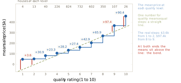
Straight lines fail in the same way well outside housing. Argonne National Laboratory modelled the fuel economy of a midsize petrol car, and Oak Ridge National Laboratory reports the results in its Transportation Energy Data Book (Davis and Boundy 2021). The car does 43 miles per gallon at 45 miles an hour, 45 at 55, 38 at 65 and 32 at 75. It rises and then falls, and no straight line in speed can do both. These are figures from a vehicle simulation rather than measurements of real cars, but the shape is the familiar one: few relationships stay straight over their whole range.
The obvious remedy, a curved model, seems to throw away everything Section 2.2 built. The projection, the normal equations and the one-step solution were all derived for predictions of the form \(\mathbf{X}\hat{\mathbf{w}}\), a weighted sum of recorded columns. The question of this section is whether a model can follow a curve and still keep that form. The answer is that it can, and the change needed is small. The model stays a weighted sum of columns, and the columns change: we compute new ones from the recorded inputs. In the terms of Definition 1.16, the slot that moves is again the hypothesis space. The loss is still the residual sum of squares of Definition 2.3, and the optimiser is still the normal equations.
A column nobody recorded
The residuals bend against quality, so the simplest repair gives the model a column that bends in quality: its square. Nobody recorded this column. It is computed row by row from one that was. For the five sales of Figure 2.35, rated 5, 6, 8, 6 and 7, the new column holds 25, 36, 64, 36 and 49 (Figure 2.59). Added to the 31 columns of the many-input fit (the ones, area, quality, year built and 27 neighbourhood indicators), it gives 32, and least squares on all 2,924 sales raises \(R^2\) from 0.823 to 0.847.
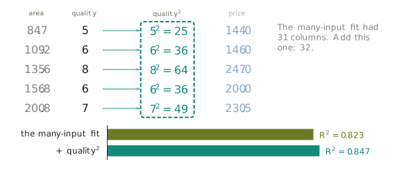
The fitted weights on the two quality columns are \(\hat{w}_q = -39.13\) and \(\hat{w}_{q^2} = 5.000\), in thousands of dollars. With every other input held fixed, the predicted price as a function of quality is a parabola, and the step it takes from level \(q\) to level \(q + 1\) follows from expanding the square:
\[ \hat{w}_q\,(q + 1) + \hat{w}_{q^2}(q + 1)^2 - \hat{w}_q\,q - \hat{w}_{q^2}\,q^2 \;=\; \hat{w}_q + \hat{w}_{q^2}\,(2q + 1) . \tag{2.46}\]
Each step is larger than the one before by \(2\hat{w}_{q^2} = 10.0\) thousand dollars. The squared column has replaced the claim of equal steps with the claim of steps that grow at a constant rate. The step from 8 to 9 is \(-39.13 + 5.000 \times 17 = 45.9\) thousand dollars, and the step from 9 to 10 is 55.9. At the bottom of the scale the formula gives a step of \(-24.1\) from 1 to 2: the parabola turns at \(q = 39.13 / 10.0 = 3.9\) and predicts that a house rated 1 is worth more than an otherwise identical house rated 2.
Figure 2.60 shows both effects. On the left, the house held back since Section 2.1, rated 5, is priced as its quality varies with its other inputs fixed. The straight line of Section 2.2 and the new curve nearly agree at the house itself, $154.0 thousand and $152.1 thousand against a sale price of $163.0 thousand, and part company at the ends. On the right are the mean residuals at each level. At quality 10 the miss falls from $87.5 thousand to $33.1 thousand, so the bend at the top is more than halved. At quality 1 it moves from \(+27.7\) to \(-85.1\). Only four houses are rated 1, so they count for little in the RSS, and the curve that straightens the top overshoots the bottom. A square is one curve for the whole range, and moving one end moves the other. The powers, under Three families of columns below, show why.
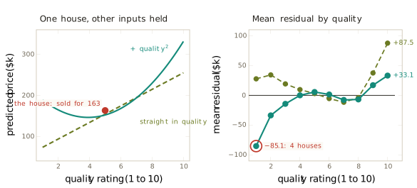
Linear in the weights
The model now draws a curve, and it was fitted with the formula of Section 2.2, which was derived for linear models. Both statements are true because the word linear has to be read with care. As a function of quality the prediction is a parabola, which is not linear. As a function of the weights it is. Fix one house and vary a single weight, say \(\hat{w}_{q^2}\), while holding the others. For that house the column \(q^2\) is one fixed number, 25 for our house, so the prediction is a constant plus \(\hat{w}_{q^2}\) times 25. It moves along a straight line (Figure 2.61).
Definition 2.26 (Linear in the weights) A model is linear in its weights when its prediction is a weighted sum of columns that can be computed from the inputs before the fit, so that every weight only multiplies a column.
The definition separates two models that look alike. The quadratic \(\hat{y} = \hat{w}_0 + \hat{w}_1 q + \hat{w}_2 q^2\) is a weighted sum of the columns \(1\), \(q\) and \(q^2\). The exponential \(\hat{y} = \hat{w}_0\, e^{\hat{w}_1 q}\) puts a weight in the exponent, and no column computed before the fit can hold it. The difference shows in the derivatives that Section 2.1 used to find the bottom of the RSS. For a model linear in its weights,
\[ \frac{\partial \hat{y}_i}{\partial \hat{w}_j} \;=\; x_{ij} , \tag{2.47}\]
the entry at observation \(i\) of the column that \(\hat{w}_j\) multiplies. That column was computed before the fit, so the entry is a number that does not depend on any weight. (For a built column, the next part writes this entry \(\phi_j(\mathbf{x}_i)\).) Every partial derivative of the RSS is then a linear expression in the weights, by Equation 2.39, and setting them all to zero gives linear equations: the normal equations. For the exponential model, \(\partial \hat{y}_i / \partial \hat{w}_1 = \hat{w}_0\, q_i\, e^{\hat{w}_1 q_i}\) depends on both weights, and setting the derivatives to zero gives equations with no general solution in closed form.
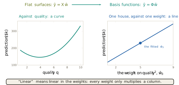
The test is quick to apply. The model \(w_0 + w_1 \log x\) is linear in its weights, because \(\log x\) is a column we can compute before the fit. So is \(w_0 + w_1 \max(0, x - 7)\), whose column is zero until \(x\) passes 7 and then rises with it. The model \(w_0 + w_1 \max(0, x - k)\), with the bend point \(k\) a parameter to be fitted as well, is not: the column cannot be computed until \(k\) is known, and \(k\) sits inside it. This last model returns at the end of the section.
The four families of Equation 2.1, which Section 2.1 treated as four kinds of model, are now one kind. Each is a weighted sum of columns, and the families differ only in which columns are allowed:
\[ \begin{aligned} &\text{constant:} && 1, \\ &\text{linear:} && 1,\ x, \\ &\text{quadratic:} && 1,\ x,\ x^2, \\ &\text{higher order:} && 1,\ x,\ x^2,\ \ldots,\ x^d . \end{aligned} \tag{2.48}\]
All four are linear in their weights, and all four are fitted by the same normal equations. Choosing among them is no longer a choice of method. It is a choice of how many columns to build, one, two, three or \(d + 1\), and that number can be turned like a dial.
Basis functions and the matrix \(\boldsymbol{\Phi}\)
Every model that passed the test is a weighted sum of columns, each computed from the recorded inputs by a fixed rule. The rule deserves a name.
Definition 2.27 (Basis function) A basis function \(\phi_j(\mathbf{x})\) is a fixed rule that computes one number from an observation’s recorded inputs \(\mathbf{x}\). With \(\phi_0(\mathbf{x}) = 1\) and \(m\) basis functions besides it, the basis matrix \(\boldsymbol{\Phi}\) has one row per observation and one column per basis function, so that its shape is \(n \times (m + 1)\) and its entry in row \(i\) and column \(j\) is \(\phi_j(\mathbf{x}_i)\).
Row \(i\) of \(\boldsymbol{\Phi}\) is observation \(i\) put through every basis function, the vector \(\boldsymbol{\phi}(\mathbf{x}_i)\) laid on its side, \(\boldsymbol{\phi}(\mathbf{x}_i)^\top\). For the five sales with \(\phi_0 = 1\), \(\phi_1 = \text{area}\), \(\phi_2 = q\) and \(\phi_3 = q^2\), \(\boldsymbol{\Phi}\) is \(5 \times 4\) (Figure 2.62). For all of Ames, with the 31 columns of the many-input fit and quality squared, it is \(2{,}924 \times 32\). The design matrix \(\mathbf{X}\) of Definition 2.15 is the special case in which every basis function returns one recorded input unchanged, and \(m\) plays the part that \(p\) played there.
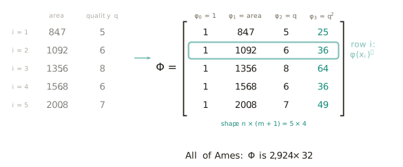
The true model and its estimate keep the form of Equation 2.33, with \(\boldsymbol{\Phi}\) in place of \(\mathbf{X}\):
\[ \mathbf{y} \;=\; \boldsymbol{\Phi}\mathbf{w} + \boldsymbol{\varepsilon}, \qquad\qquad \hat{\mathbf{y}} \;=\; \boldsymbol{\Phi}\hat{\mathbf{w}} . \tag{2.49}\]
For one observation the prediction is \(\hat{y} = \sum_{j=0}^{m} \hat{w}_j\, \phi_j(\mathbf{x})\), which is a curve in the inputs whenever the basis functions are curves, and a weighted sum all the same.
Nothing in the argument of Section 2.2 has to be repeated, and the reason is worth stating. The projection argument used three facts: every prediction \(\mathbf{X}\hat{\mathbf{w}}\) is a combination of the columns (Equation 2.30), the RSS is the squared length of \(\mathbf{y} - \mathbf{X}\hat{\mathbf{w}}\) (Equation 2.32), and a residual orthogonal to every column gives the closest point (Equation 2.34). None of them asked what a column holds. A column of areas, of squared ratings or of hinges is a list of \(n\) numbers, an arrow in the space of houses, and the shadow of \(\mathbf{y}\) on the span of those arrows is found in the same way (Figure 2.63). The normal equations therefore carry over word for word,
\[ \boldsymbol{\Phi}^\top\boldsymbol{\Phi}\,\hat{\mathbf{w}} \;=\; \boldsymbol{\Phi}^\top\mathbf{y}, \qquad\qquad \hat{\mathbf{w}} \;=\; (\boldsymbol{\Phi}^\top\boldsymbol{\Phi})^{-1}\,\boldsymbol{\Phi}^\top\mathbf{y} , \tag{2.50}\]
the second whenever \(\boldsymbol{\Phi}\) has full column rank (Definition 2.22). The conditions of Section 2.2 carry over with them. A built column that is a combination of others breaks the rank exactly as a repeated recorded column did. The square of a column that takes only the values 0 and 1 is an example: it equals the column itself, so a model that holds both has the same column twice.
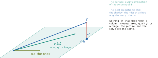
The basis functions decide something the solver does not. Fix the columns \(1\), \(q\) and \(q^2\). Each choice of weights draws one member of a family of parabolas, and Figure 2.64 draws several. Read at the recorded houses, each member is a vector of predictions \(\boldsymbol{\Phi}\hat{\mathbf{w}}\), a combination of the three columns, and every such combination is some member. The family, read at the data, is therefore exactly the span of Definition 2.16. Least squares picks one member of it, the one whose predictions are the shadow of the prices. Section 1.3 introduced the hypothesis space \(\mathcal{H}\) as the set of candidate functions worth considering. For a model linear in its weights that set can now be written down:
\[ \mathcal{H} \;=\; \Bigl\{\, f(\mathbf{x}) = \sum_{j=0}^{m} w_j\,\phi_j(\mathbf{x}) \;:\; w_0, \ldots, w_m \text{ any numbers} \Bigr\} , \tag{2.51}\]
and on the recorded observations it is the span of the columns of \(\boldsymbol{\Phi}\). To choose the basis functions is to choose the hypothesis space.
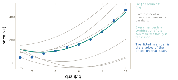
Definition 2.28 (Feature construction) Feature construction is computing new input columns from the recorded ones, through basis functions chosen by the modeller. For a model linear in its weights it is a choice of hypothesis space.
Three families of columns
If the columns decide the hypothesis space, the practical question is which columns are worth building. Three families cover most of what a modeller does by hand, and each makes a different claim about the world.
Powers. The columns \(1, q, q^2, q^3, \ldots\) are defined over the whole range of the input (Figure 2.65, left), and a weighted sum of them is one smooth curve. That is their strength and their weakness. Fit quality alone with its square, \(\hat{y} = 149.6 - 37.68\,q + 6.666\,q^2\), and the curve follows the steep rise at the top of the scale. To do so it lifts the bottom: at quality 1 it predicts $118.6 thousand, about $70 thousand above the mean price of $48.7 thousand. The reason is that a power column is global. Raise the weight on \(q^2\) by one and every prediction rises by \(q^2\): by 4 at quality 2, by 25 at quality 5 and by 64 at quality 8 (Figure 2.65, right). No weight of a polynomial moves one part of the curve alone, and this is the overshoot of Figure 2.60 explained.
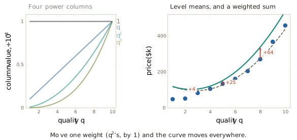
Fitting a polynomial by least squares goes back more than two centuries. Gergonne published, in 1815 in the Annales de Mathématiques Pures et Appliquées, a paper applying least squares to polynomial interpolation (Gergonne 1815). Stigler brought it back to notice in Historia Mathematica in 1974, beside an English translation in the same issue, and read it as an early paper on the design of experiments for polynomial regression (Stigler 1974). The method assumes that the relationship bends smoothly and in the same way along the whole range of the input.
One column per level. Quality takes ten values, and each can have its own indicator column (Definition 2.20), exactly as the neighbourhoods did. With the ones column present, one level is dropped to avoid the trap of Section 2.2, here quality 1, which becomes the reference. Fitted to quality alone, the model gives every level its own price, and the normal equations show that the price is the level mean. The equation for the ones column says that the residuals sum to zero over all sales. The equation for the indicator of level \(j\) says that they sum to zero over the sales at level \(j\). Subtracting the nine indicator equations from the first leaves the same statement for the reference level. Every level’s residuals therefore sum to zero, which for a model that predicts one number per level means that the number is the level’s mean.
The same argument holds in the full fit, where area, year built and neighbourhood are present as well, since it uses only the equations of the ones column and the indicators. Replacing the single quality column by nine level indicators raises \(R^2\) from 0.823 to 0.859, and every level’s mean residual becomes exactly zero (Figure 2.66). The fitted shifts against quality 1, with the other inputs held, are 26.8, 32.6, 43.3, 54.5, 63.7, 77.1, 114.1, 186.9 and 259.4 thousand dollars for levels 2 to 10. The steps between them, computed before rounding, are 26.8, 5.9, 10.6, 11.2, 9.2, 13.4, 37.0, 72.8 and 72.5. These are not the steps of Figure 2.58, which compare the mean prices of houses that also differ in area, age and neighbourhood. Here those inputs are held fixed. The first step rests on the 17 houses rated 1 or 2 and is poorly determined. The others are close to equal through the middle of the scale and grow sharply above level 7. With quality as its only input the comparison is starker still: one column gives \(R^2 = 0.648\), the column and its square 0.704, and one column per level 0.714. The evidence against equal steps is the fitted steps themselves, which assume nothing about one another and come out far from equal. The rise in \(R^2\) is not evidence, because adding columns can only raise it, as The capacity dial below shows. The price of the freedom is nine weights where one served before, and with them nine numbers the data must determine.
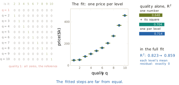
Two bases can build the same hypothesis space. Fit quality alone with the ten power columns \(1, q, \ldots, q^9\) and the result is \(R^2 = 0.7142\), the value for the ten level columns to four figures. The two fits are the same fit. Quality takes only ten values, and on ten distinct values a polynomial of degree 9 can be made to take any ten numbers we choose (exercise 6). In particular, some polynomial of degree 9 equals 1 at quality 2 and 0 at the other nine levels, and that polynomial, read at the sales, is the indicator of level 2. Each set of ten columns builds every column of the other, so both have the same span, the same shadow and the same predictions. Between the levels the polynomial swings, with a dip below the level-1 mean between quality 1 and 2, but no house has a rating there, so no prediction lands on it.
Hinges. A power bends everywhere at once. Often the bend belongs in one place.
Definition 2.29 (Hinge function) A hinge function with knot \(k\) is \[ h_k(x) \;=\; \max(0,\ x - k) , \tag{2.52}\] which is zero for \(x \le k\) and rises with slope 1 beyond the knot.
With the knot fixed, \(h_k\) is an ordinary column, and the model \(\hat{w}_0 + \hat{w}_1 q + \hat{w}_2\, h_7(q)\) is linear in its weights. It draws two straight pieces joined at the knot, with slope \(\hat{w}_1\) to the left and \(\hat{w}_1 + \hat{w}_2\) to the right. Changing \(\hat{w}_2\) changes nothing to the left of the knot (Figure 2.67, right), and that is the difference from a power: a hinge is local. Added to the many-input fit with the knot at 7, it raises \(R^2\) from 0.823 to 0.855, and the fitted slope in quality is $10.2 thousand per point up to level 7 and $53.3 thousand per point above it. The knot at 7 was chosen by trying 5, 6, 7 and 8, which give 0.828, 0.840, 0.855 and 0.853. The choice was ours, made by search, and it was made outside the normal equations. Each of the four candidates adds one column, so the comparison is between spaces of the same size, but it is still made on the sales the fit was trained on, and The capacity dial below shows how far such a score can mislead.
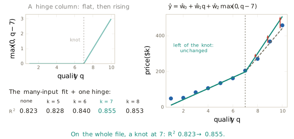
Pieces joined at knots have a name. Schoenberg, in a two-part paper on the approximation of equally spaced data published in the Quarterly of Applied Mathematics in 1946 (Schoenberg 1946), called them splines: polynomial pieces joined smoothly at knots. The name comes from the flexible strips that draughtsmen bent through fixed points to draw smooth curves. A sum of hinges is the simplest spline, made of straight pieces. The method assumes that the bends sit at knots chosen in advance.
Products. The second hidden assumption of Section 2.2 was that a square metre is worth the same at every level of quality. A column that is the product of two inputs removes it.
Definition 2.30 (Interaction column) An interaction column is the product of two input columns. Its weight lets the effect of each input depend on the value of the other.
Fitted to area, quality and their product, the model is
\[ \hat{y} \;=\; 96.0 \;-\; 0.860\,\text{area} \;-\; 1.297\,q \;+\; 0.240\,\text{area}\cdot q , \tag{2.53}\]
in thousands of dollars, with \(R^2 = 0.801\) against 0.751 for area and quality without the product. Holding quality at a fixed level and collecting the terms in area gives the price of one square metre,
\[ \frac{\partial \hat{y}}{\partial\,\text{area}} \;=\; -0.860 + 0.240\,q , \tag{2.54}\]
which is no longer a constant. A square metre adds $101 at quality 4, $582 at quality 6 and $1,062 at quality 8, about ten times as much in a well-built house as in a modest one. These figures use the unrounded weights. The parallel lines of Figure 2.29 fan out (Figure 2.68). For a house rated 9 the slope is \(-0.860 + 9 \times 0.240 = 1.300\) thousand dollars per square metre, so ten more square metres add $13.0 thousand, where the parallel lines of Section 2.2 added $6.8 thousand at every level.
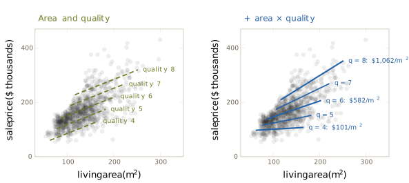
The product changes the meaning of the other weights. By the same reasoning, the effect of one quality point is \(-1.297 + 0.240\,\text{area}\), which is $30.8 thousand for the held-back house of 133.8 square metres. The weight \(-1.297\) on its own is the effect of quality on a house with no floor area. No such house exists, and the weight is not to be read as the effect of quality. A weight in a model with interaction columns describes one input at a stated value of the other.
Columns of different families can be combined. With both quality squared and the product, the flat surface of Figure 2.28 bends along quality and twists along area, and it remains a weighted sum of five columns (Figure 2.69).
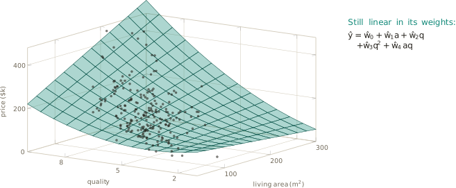
Figure 2.70 collects the built columns on the whole file. The many-input fit gives 0.823. Quality squared raises it to 0.847, and the product to 0.858. Replacing quality by its levels gives 0.859, and the product area \(\times\, q\), with \(q\) the rating as a number, added to the levels 0.868. Every column changed the span, and every change raised the score on these sales. Section 2.2 placed indicators and standardising among the work of preparing data, a stage before the model. Standardising belongs there, since it leaves the span unchanged and so changes no prediction. A built column does not belong there. It enlarges the span and so changes what the model can draw, which makes it part of the hypothesis space, as Definition 2.28 says.
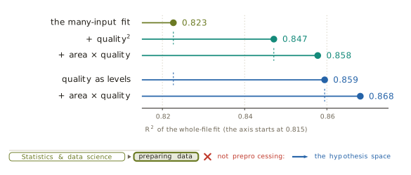
The capacity dial
Every column helped, which raises the question of what happens when we keep adding them. Quality is the wrong input for the experiment. It takes ten values, so a curve in quality has nowhere to go between them, and ten columns already fit the ten means exactly. We return to the thirty typical sales of Section 2.1, one from the middle of each thirtieth of the houses by size, and fit polynomials in living area of increasing degree \(d\). Area is standardised first, for a reason given at the end of this part.
| degree \(d\) | 0 | 1 | 2 | 3 | 4 | 5 | 8 | 12 | 15 | 20 | 25 | 29 |
|---|---|---|---|---|---|---|---|---|---|---|---|---|
| training RSS | 71,202 | 5,514 | 3,945 | 3,054 | 3,025 | 3,022 | 2,787 | 2,153 | 1,807 | 1,000 | 439 | 0 |
Degree 0 is the mean price alone, and its RSS of 71,202 is the total variation of the thirty prices. The straight line leaves 5,514, so \(R^2 = 0.923\) on these well-spread sales. From there the RSS keeps falling (Table 2.2). It never rises, and the projection of Section 2.2 says why it cannot.
Every polynomial of degree 3 is a polynomial of degree 4 whose last weight is zero. The hypothesis space of degree 3 therefore lies inside that of degree 4, which lies inside that of degree 5, and so on. Hypothesis spaces with this property are called nested. Read at the data, each span contains the one before it, and the closest point of a larger set can be no further from \(\mathbf{y}\) than the closest point of a smaller one. The RSS cannot rise from one degree to the next. This is the argument that Section 2.2 gave for the bars of Figure 2.54, now drawn as a curve (Figure 2.71).
Definition 2.31 (Capacity) The capacity of a hypothesis space is its ability to fit the data it is trained on. Along a sequence of nested hypothesis spaces capacity can only grow, and so the training RSS can only fall.
This section uses the word only to compare nested spaces, where a space that contains another has at least its capacity. For the polynomials here that order is simply the number of columns.
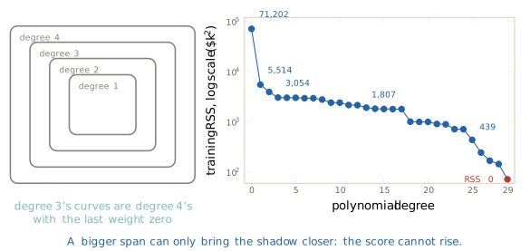
At degree 29 the RSS is zero. The model then has thirty columns for thirty houses, so \(\boldsymbol{\Phi}\) is square. The thirty areas are all different, and a polynomial of degree 29 can take any thirty values at thirty distinct points, so \(\boldsymbol{\Phi}\) has full rank and an inverse. The weights \(\boldsymbol{\Phi}^{-1}\mathbf{y}\) give predictions equal to the prices: the span is the whole space, and the shadow of \(\mathbf{y}\) is \(\mathbf{y}\) itself. A fit with as many free weights as observations interpolates, passing through every point (Figure 2.72).
Weierstrass showed in 1885, in the Sitzungsberichte of the Prussian Academy of Sciences in Berlin (Weierstrass 1885), that any continuous function on a closed interval can be approximated by polynomials as closely as we like. His assumptions were continuity and a closed, bounded interval. In the language of this section the result says that the dial has no top: by raising the degree, polynomials can follow any continuous relationship as closely as we wish. Capacity is never the obstacle.
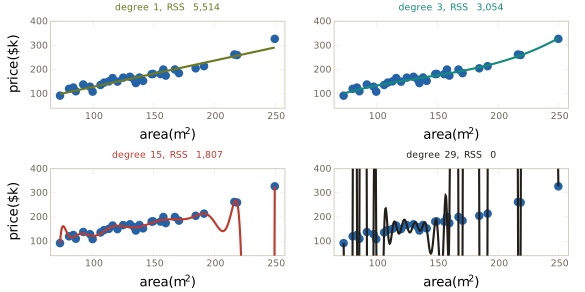
The score improves at every step, and Figure 2.72 shows that the curves do not. Degree 15 scores 1,807 against degree 3’s 3,054. Between the two largest sales, at 218.6 and 249.6 square metres, it plunges, and at 244.5 square metres it prices a house at about \(-\$37\) million (Figure 2.73). Degree 3 prices the same house at a sensible figure. The better training score belongs to the absurd price.
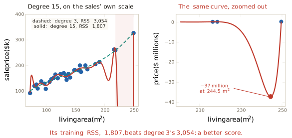
The behaviour has a history. Runge showed in 1901, in the Zeitschrift für Mathematik und Physik (Runge 1901), that polynomials of high degree passed through points spaced evenly along an interval can swing ever more wildly near its ends as the degree grows. His points were evenly spaced, and the thirty sales are not, but they swing hardest at the edge of the data all the same, where the points thin out. The same effect appeared at small scale in Section 2.1, where the straight, quadratic and cubic fits disagreed by $69 thousand beyond the largest house sold (Figure 2.3). Here it reaches millions.
The training score cannot choose the degree. It always prefers more capacity, and it is blind to what a curve does between and beyond the points it was fitted to. Choosing the degree needs data the fit has not seen, which is the subject of Section 2.7.
High powers have a second cost, which concerns the computation rather than the predictions. Over the thirty sales, area and area squared lie almost on a straight line, with a correlation of 0.985 (Figure 2.74, left). They are nearly repeated columns of the kind Section 2.2 met with the two garage columns, and nearly repeated columns make the weights unstable. Standardising area before raising it to powers helps a great deal: the standardised area and its square have a correlation of 0.48, because squaring a column centred on zero folds its negative half onto its positive half (Figure 2.74, right). If the areas were spread symmetrically about their mean the correlation would be zero. The 0.48 that remains comes from the larger houses, which stretch the positive side further than the smaller ones stretch the negative. Standardising does not solve the problem. The columns of a standardised polynomial of degree 15 still nearly repeat, and the computation strains. The condition number of a matrix measures how much a small change in the data can be magnified in the computed weights. For the \(30 \times 16\) matrix \(\boldsymbol{\Phi}\) of the standardised polynomial of degree 15 it is about \(10^9\), against about \(2.5 \times 10^5\) for the \(30 \times 3\) matrix of the raw columns \(1\), area and area². Section 2.4 defines the condition number and measures what it costs. The effect is visible without the definition. Fitting the thirty sales with NumPy’s standard least-squares routine in ordinary double-precision arithmetic, the RSS stops falling and rises at degree 22, which nested spans forbid: the computation has failed, not the mathematics. Forming the normal equations and solving them directly fails sooner, at degree 17. The figures of this section were computed with columns made exactly orthogonal to one another, which span the same space as the powers and so give the same fit, and, for the curves between the sales, in 120-digit arithmetic.
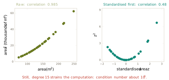
The three choices of Definition 1.16 can now be filled for this section (Figure 2.75). The hypothesis space is the span of the columns we build: powers, levels, hinges and products. The loss is the residual sum of squares, unchanged. The optimiser is the normal equations, unchanged except that \(\boldsymbol{\Phi}\) stands where \(\mathbf{X}\) stood. One slot moved, and it moved further than in any section so far, because its size became a dial. The question beneath the card is untouched, and Figure 2.73 shows that it has become pressing.
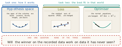
On the modelling axis of Figure 2.7, the straight line sat in the interior: its form was our assumption and its two numbers were the data’s. Raising the degree moves the method towards the black end (Figure 2.76). With more columns, less of the form is ours and more is decided by the data. Even degree 29 keeps one claim of ours, that the price is a polynomial in area, so the path stops short of the black end.
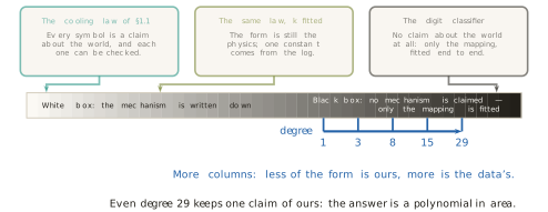
What the method assumes, and where it fails
The assumptions of Section 2.1 and Section 2.2 remain: only the price is in error, misses are judged by their squares, and the sales stand for the houses to be priced. Building columns adds assumptions of its own, one per column, and each column states a claim about the world.
- A power claims a smooth bend, the same along the whole range of the input. Fixing the fit at one end moves it at the other, as the overshoot at quality 1 showed.
- One column per level claims nothing about the steps, and pays for that freedom with one weight per level. Levels with few observations get poorly determined weights.
- A hinge claims a change of slope at a knot chosen in advance.
- A product claims that the effect of one input changes in proportion to the other, and it changes the meaning of the separate weights.
- Every built column enlarges the span, so the training RSS can only fall. A better training score is evidence of more capacity, not of a better model.
- High powers nearly repeat one another, and the computation of their weights loses accuracy, even after standardising.
The last assumption is the one this section relied on throughout: every bend was placed by us. The knot at quality 7 was found by trying four values. Suppose instead that the data are to choose where the bend goes. On the thirty typical sales the model is
\[ y \;=\; b + w_1\,\text{area} + w_2 \max(0,\ \text{area} - k) + \varepsilon , \tag{2.55}\]
with the knot \(k\) a parameter like the others. For any fixed \(k\) the hinge column can be computed, and the normal equations give the best \(\hat{b}\), \(\hat{w}_1\) and \(\hat{w}_2\) in one solve. The smallest of the thirty sales is 72.8 square metres and the largest 249.6, so every knot from 80 up has sales on both sides of it. Repeating the solve for each \(k\) from 80 to 249.5 square metres in steps of half a square metre traces the RSS as a function of the knot (Figure 2.77). It is not a bowl. It rises briefly from \(k = 80\) to \(k = 85\), falls to one bottom at \(k = 197\) square metres, where the RSS is 3,131 against 5,514 for the straight line, and then rises to a flat stretch. The fitted slope is $901 per square metre below the knot and $2,043 above it. The flat stretch has a simple cause. For any knot between the second-largest sale, at 218.6 square metres, and the largest, at 249.6, the hinge column is zero for every sale but the largest. It then acts as an indicator of that one sale, whose weight fits it exactly, and the RSS is that of a straight line through the other 29 sales, 3,784, whatever the value of \(k\).
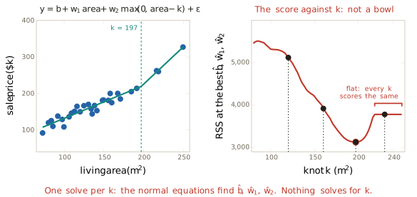
Each point of that curve is one solve, and nothing solves for \(k\) itself. The knot sits inside a basis function, and the model is no longer linear in its parameters. Equation 2.47 fails for it. The derivative of a prediction with respect to \(k\) is \(-\hat{w}_2\) for sales beyond the knot and zero for the others, so it depends on another parameter and jumps as the knot passes a sale. The normal equations, which needed every derivative to be a fixed column, cannot reach it. The closed form, which Section 2.1 found for the line and Section 2.2 extended to any number of columns, ends here, at the first model whose parameters do not all multiply columns. Finding the bottom of a score without a formula is the subject of Section 2.4. Two later developments start from the same place. Section 4.2 uses more basis functions than could ever be built as columns, without building them, and Section 6.1 lets the data choose the basis functions themselves, knots included.
Exercises
For each model, say whether it is linear in its weights \(w_0\), \(w_1\), \(w_2\), and if it is, list the columns of \(\boldsymbol{\Phi}\): (a) \(w_0 + w_1 x + w_2 x^2\); (b) \(w_0 + w_1 \log x\); (c) \(w_0\, e^{w_1 x}\); (d) \(w_0 + w_1 \max(0, x - 7)\); (e) \(w_0 + w_1 \max(0, x - k)\) with \(k\) fitted; (f) \(w_0 + w_1 \sin x + w_2 \cos x\); (g) \(w_0 + x^{w_1}\); (h) \((w_0 + w_1 x)^2\).
For the five sales of Figure 2.62, write \(\boldsymbol{\Phi}\) for the basis \(1\), area, \(q\), \(q^2\) and area \(\times\, q\), with \(q\) the rating as a number, and give its shape. Give the shapes of \(\hat{\mathbf{w}}\), \(\boldsymbol{\Phi}\hat{\mathbf{w}}\), \(\boldsymbol{\Phi}^\top\boldsymbol{\Phi}\) and \(\boldsymbol{\Phi}^\top\mathbf{y}\). Then give the shape of \(\boldsymbol{\Phi}\) for the whole-file fit with levels and the product (Figure 2.70, last bar), and explain why the dummy-variable trap of Section 2.2 does not arise when quality is entered as levels 2 to 10 beside the ones column.
Use the weights of Equation 2.53. (a) Find the price of one extra square metre at quality 5 and at quality 7. (b) Find the effect of one extra quality point for houses of 100 and 200 square metres. (c) A colleague reads the weight \(-1.297\) as “a better-built house is worth less”. Explain the error. (d) Find the area at which one quality point is worth nothing, and say whether a house of that size is a realistic case.
The fit with quality squared has \(\hat{w}_q = -39.13\) and \(\hat{w}_{q^2} = 5.000\). (a) Derive Equation 2.46. (b) Compute the steps from 1 to 2, from 4 to 5 and from 9 to 10, and find the quality at which the fitted curve turns. (c) Compare the steps with those of the level fit in the text, and explain in two or three sentences why the square overshoots at quality 1 while the levels do not.
Prove that in any least-squares fit containing the ones column and the indicator columns of a category with one level dropped as the reference, the residuals sum to zero within every level of the category, whatever other columns the model contains. Conclude that the mean residual of the level fit is exactly zero at every quality level, and explain why the fit with quality squared has no such property.
Let \(q_1, \ldots, q_{10}\) be ten distinct numbers. (a) For each \(j\), show that \(L_j(q) = \prod_{\ell \neq j} (q - q_\ell)/(q_j - q_\ell)\) is a polynomial of degree 9 that equals 1 at \(q_j\) and 0 at every other \(q_\ell\). (b) Use (a) to show that, on data whose input takes only these ten values, the span of the columns \(1, q, \ldots, q^9\) contains every level indicator, and the reverse. (c) Conclude that the two fits have the same predictions and the same \(R^2\), and say what happens if the input takes eleven values.
- Prove that the training RSS of a polynomial fit of degree \(d + 1\) is at most that of degree \(d\), on the same data. (b) Show that with \(n\) observations at distinct inputs, a polynomial of degree \(n - 1\) has training RSS zero. (c) What happens to the rank of \(\boldsymbol{\Phi}\), and to the weights, at degree \(n\) or above? (d) Explain why (a) means that the training RSS cannot be used to choose the degree, and describe what kind of evidence could be used instead.
For the thirty typical sales and the model Equation 2.55: (a) Show that for any knot \(k\) with \(218.6 \le k < 249.6\) the hinge column is a multiple of the indicator of the largest sale, and deduce that the RSS equals that of a straight line through the other 29 sales. (b) Explain why the fitted model with such a knot passes exactly through the largest sale. (c) Show that the RSS, as a function of \(k\), is continuous for knots strictly between the smallest and the largest sale, and say what happens at the two ends. Show that it cannot be minimised by setting a derivative of the normal-equations kind to zero, and say what any method that finds the best \(k\) must do instead.